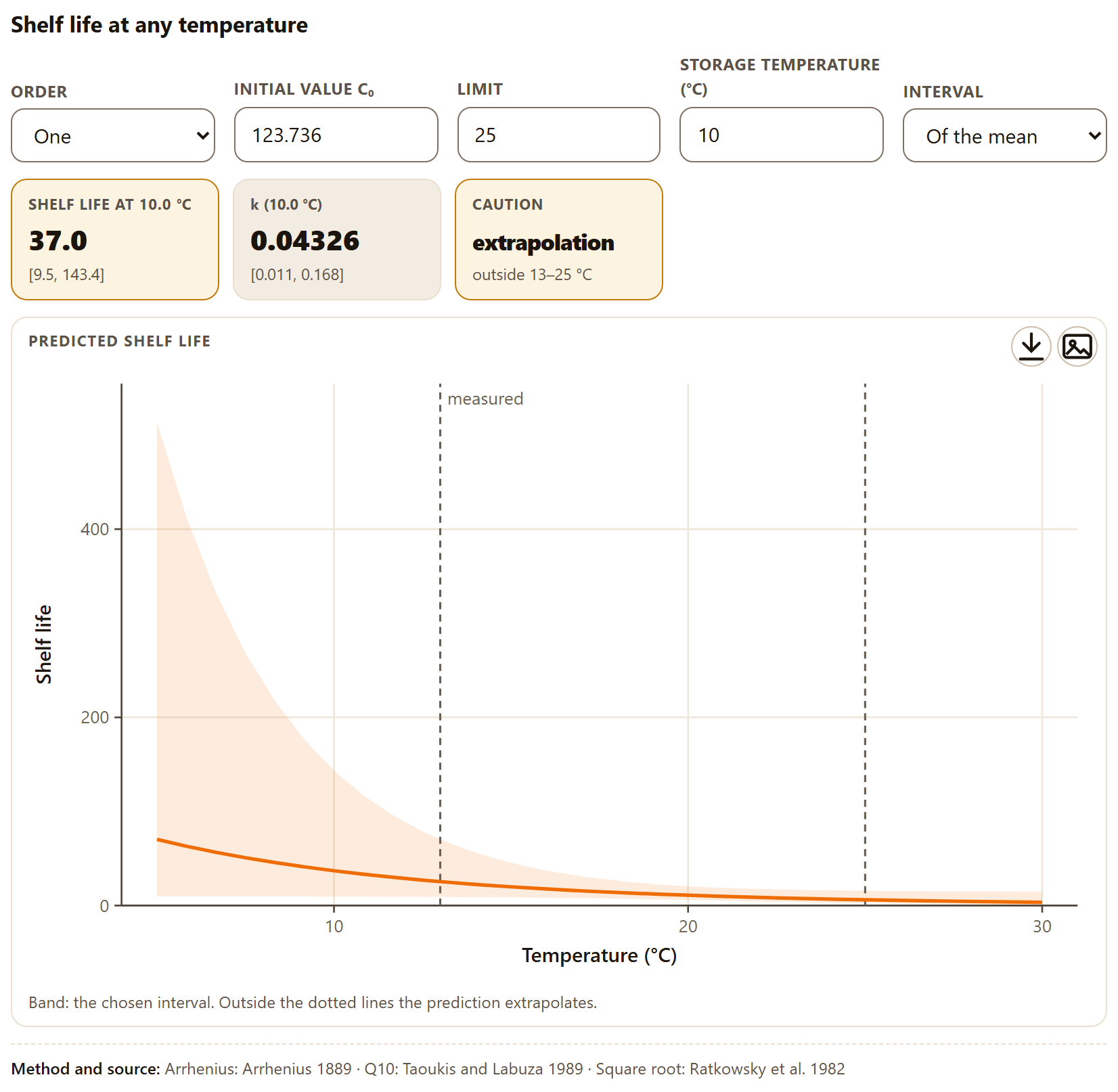
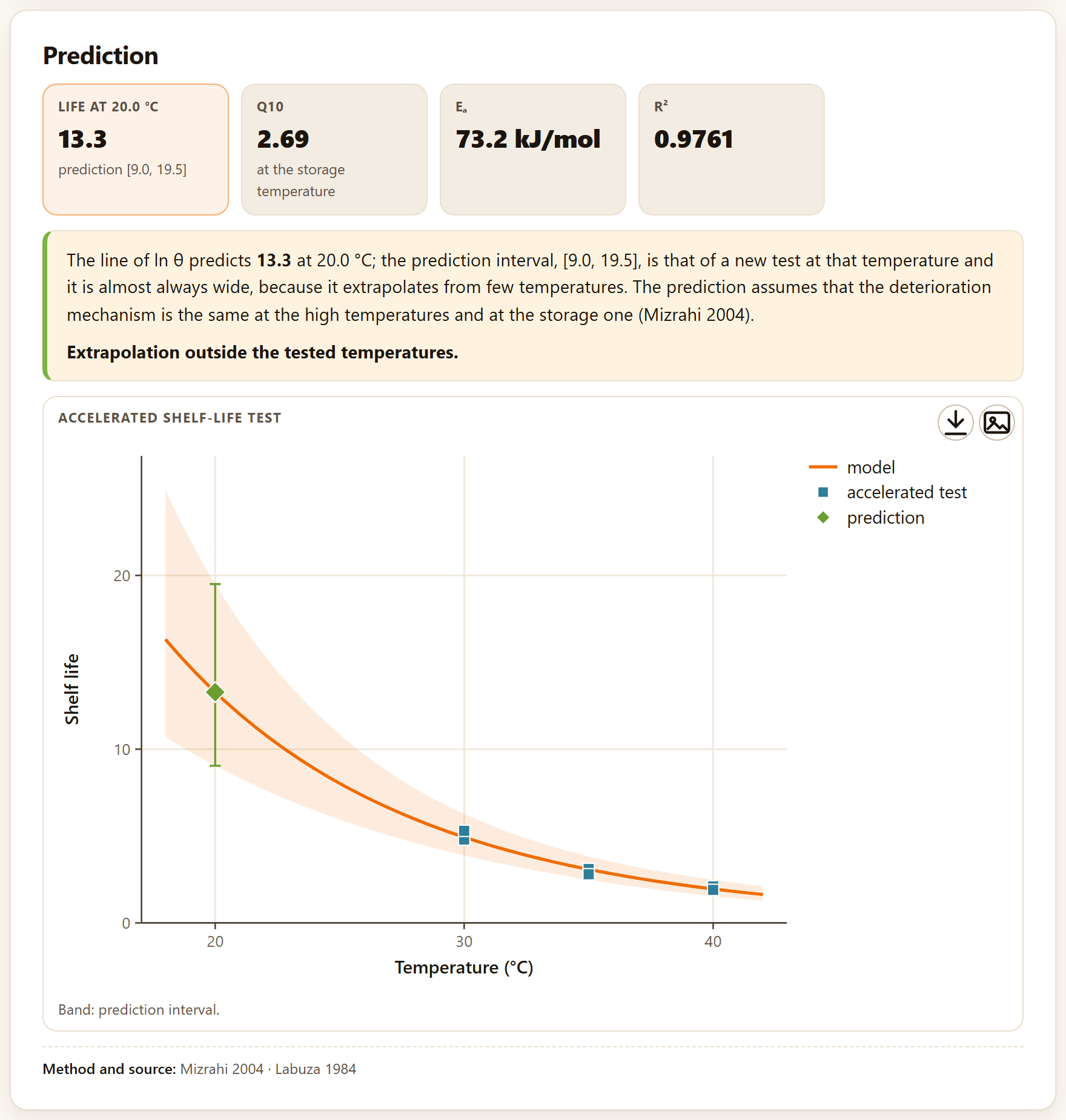
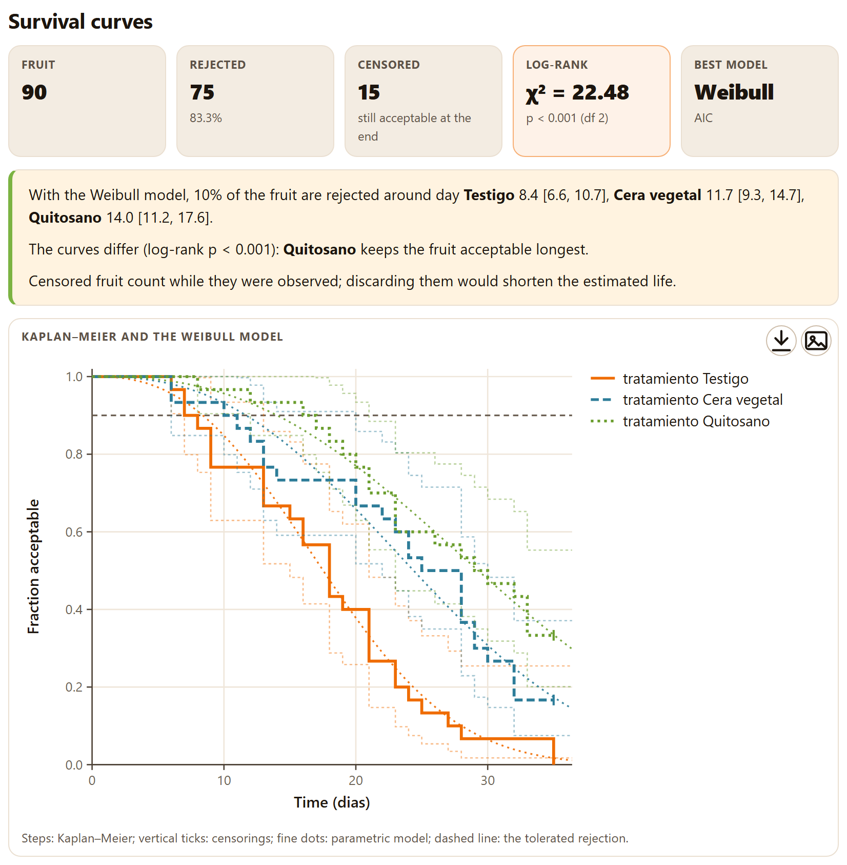
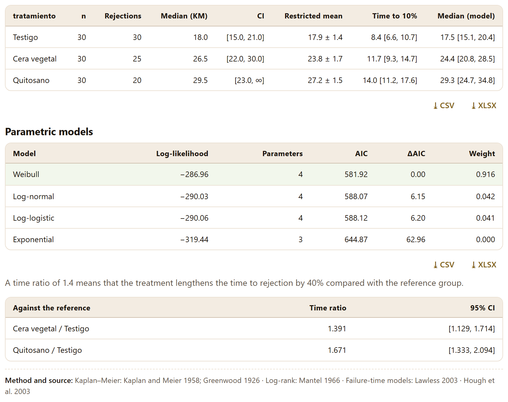
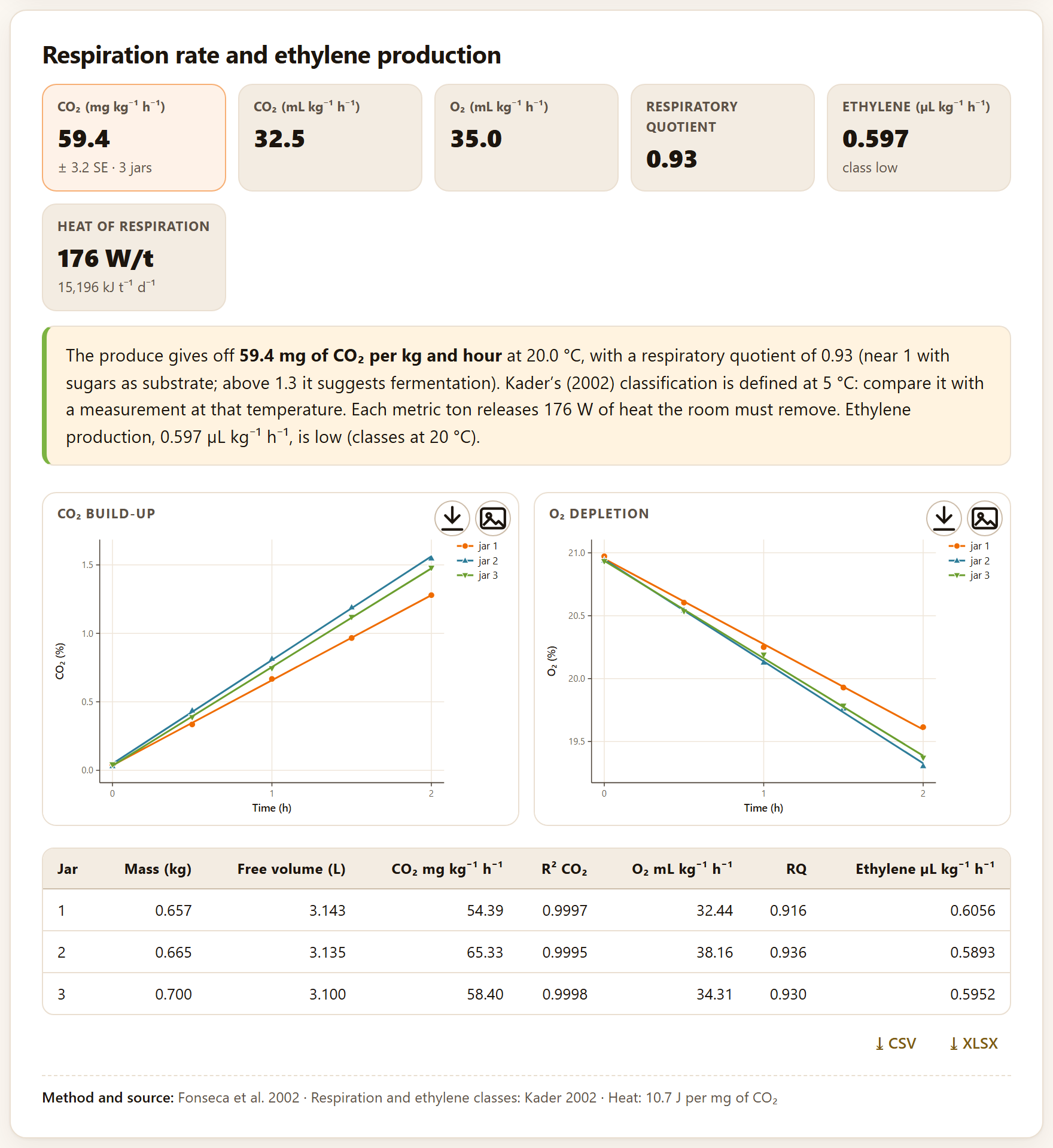
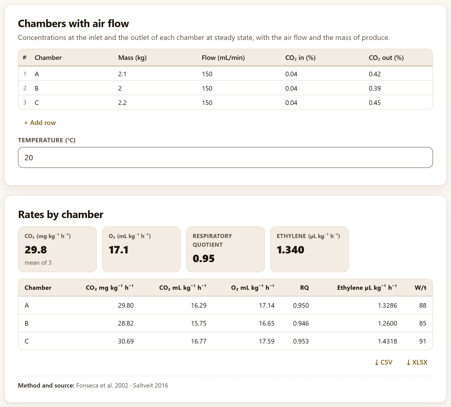
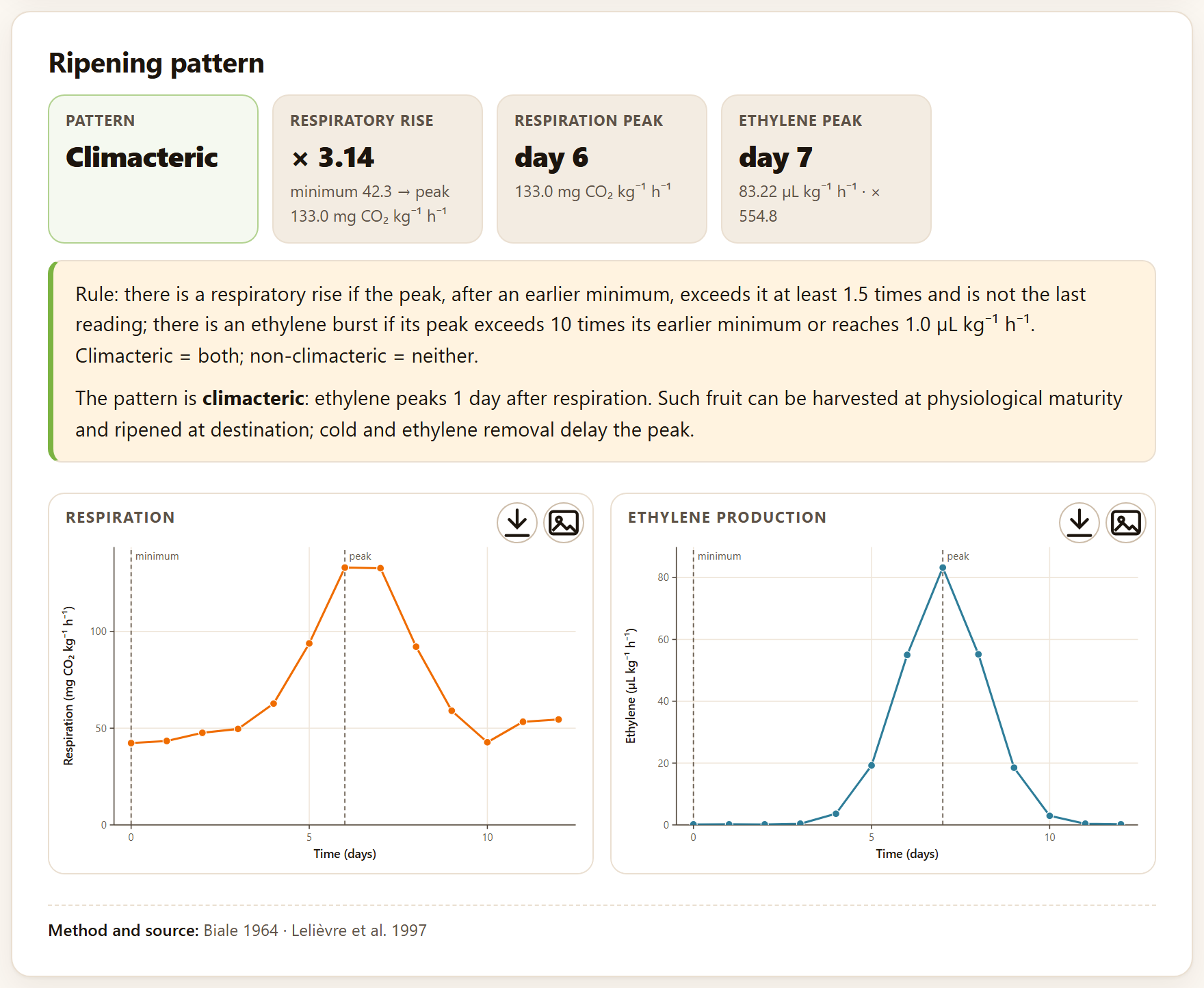
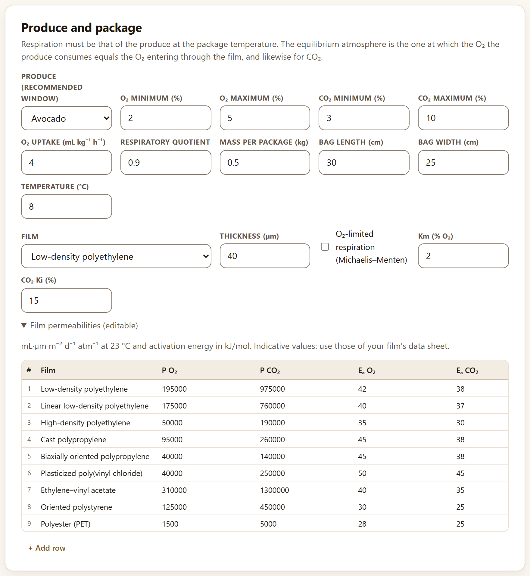
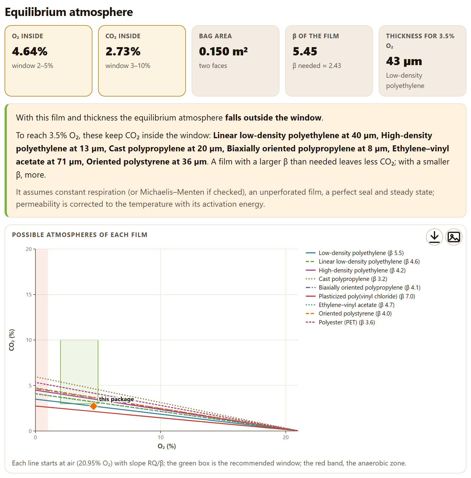
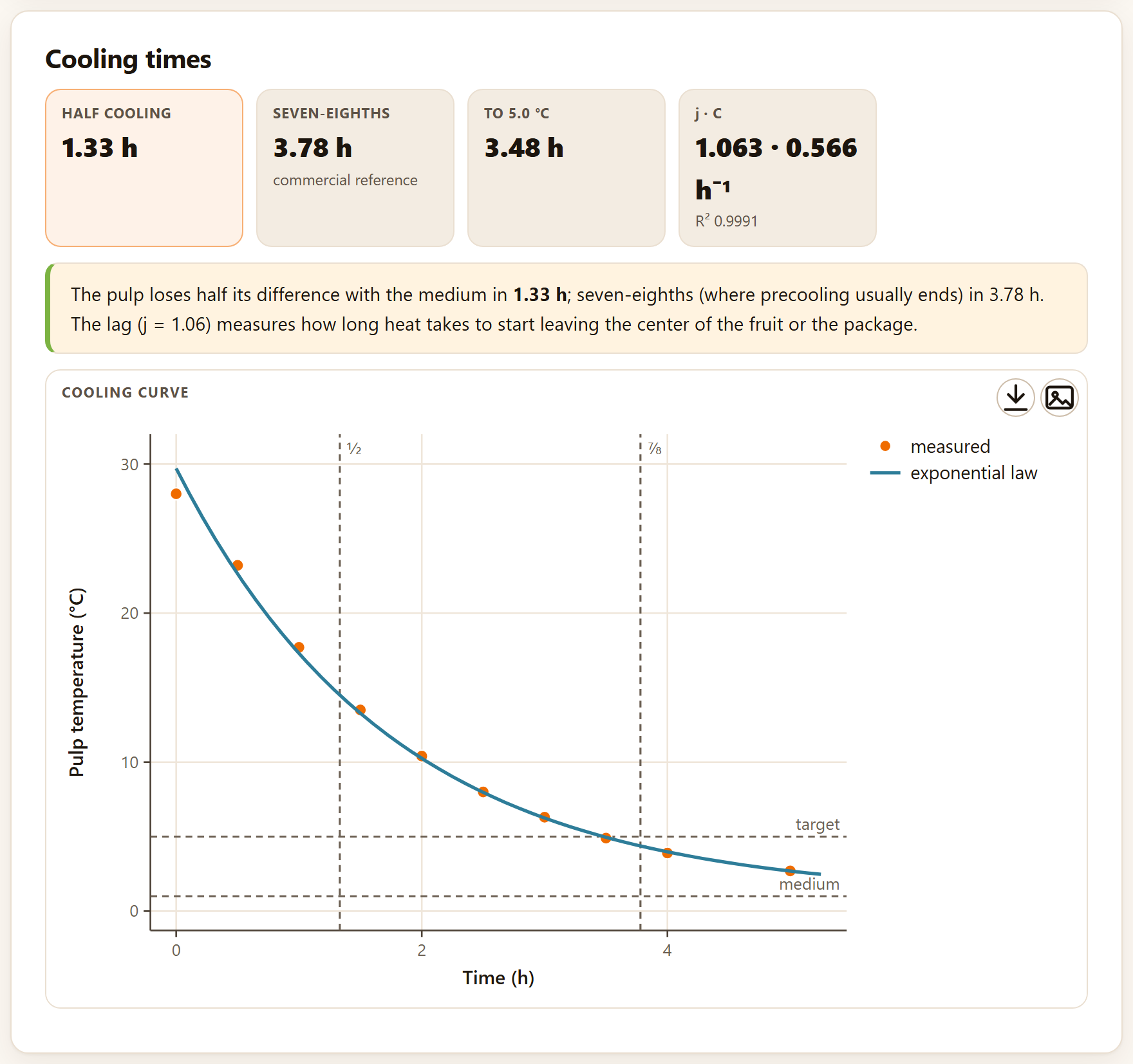
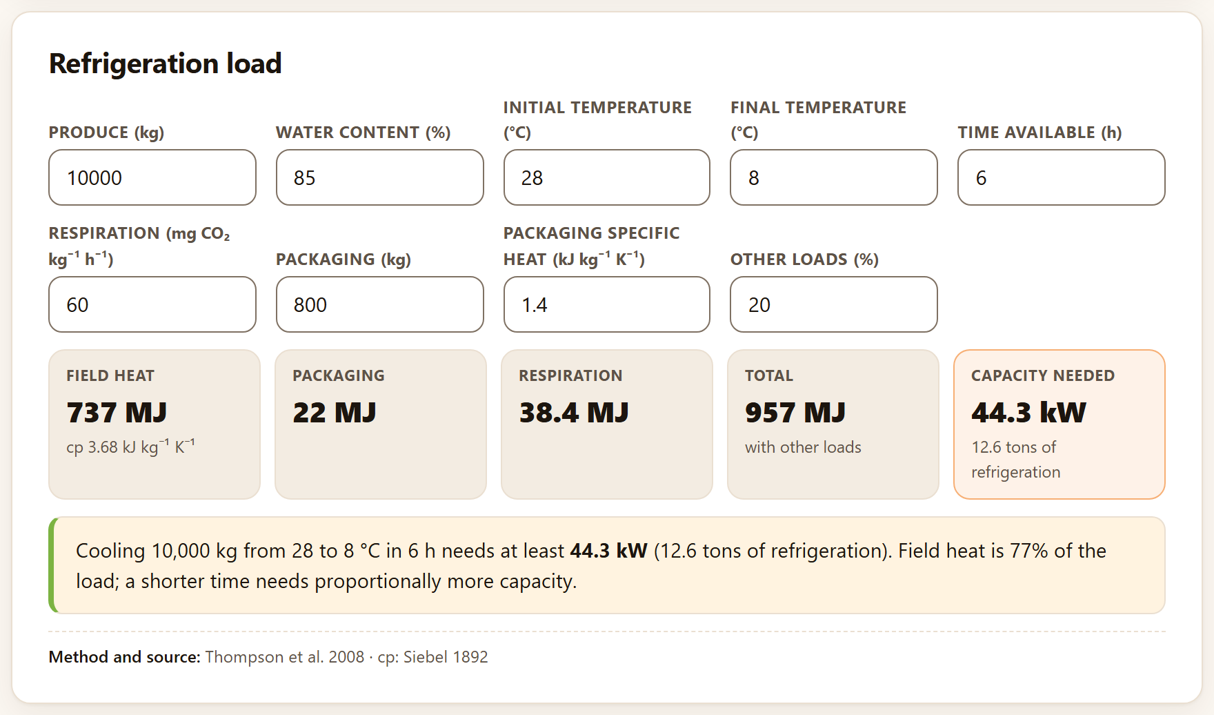
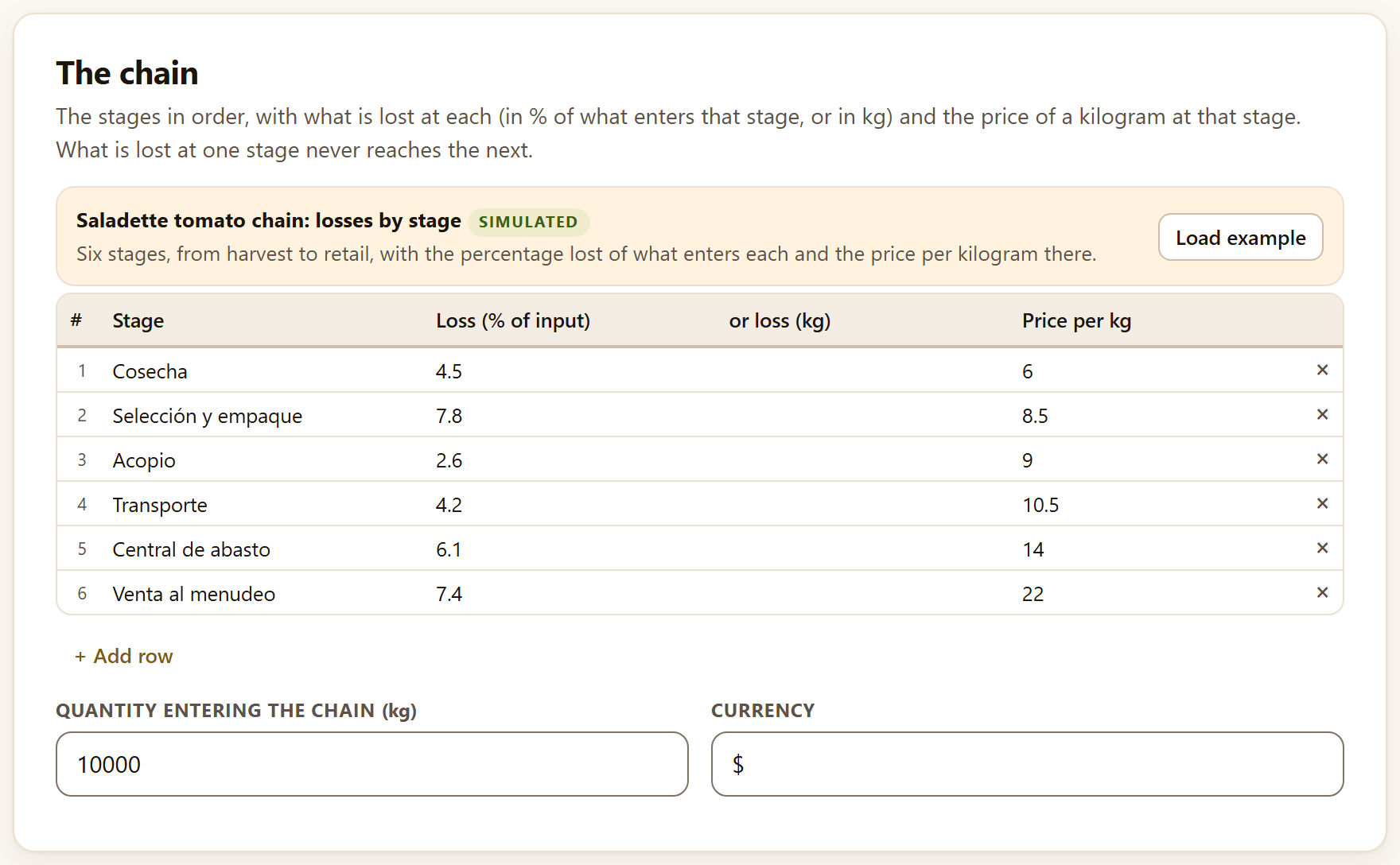
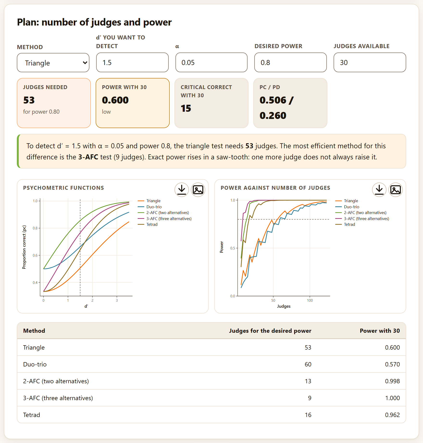
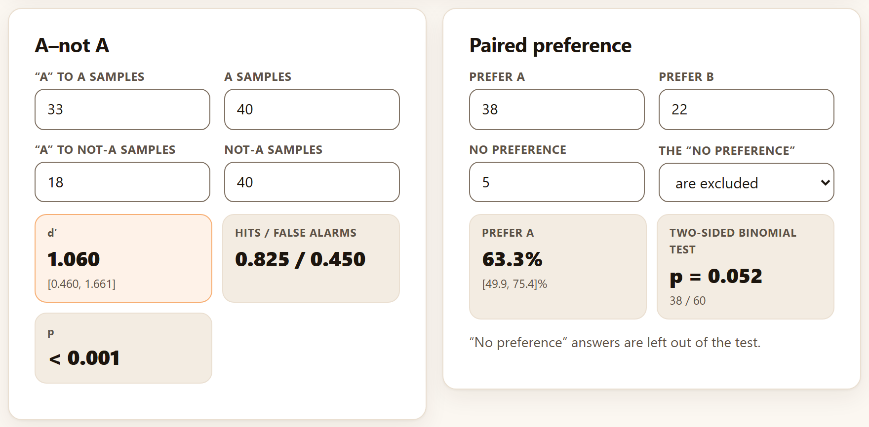
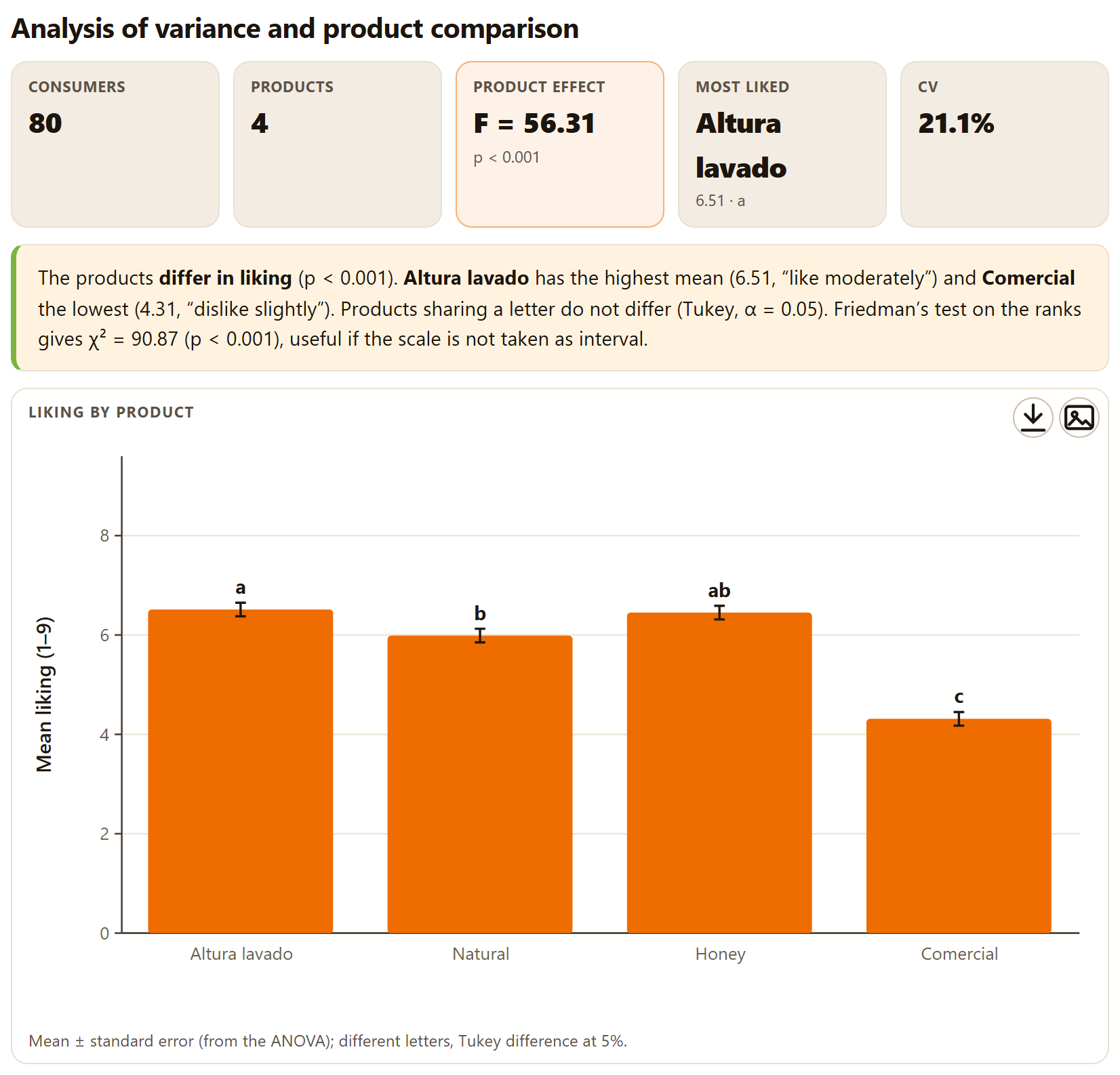
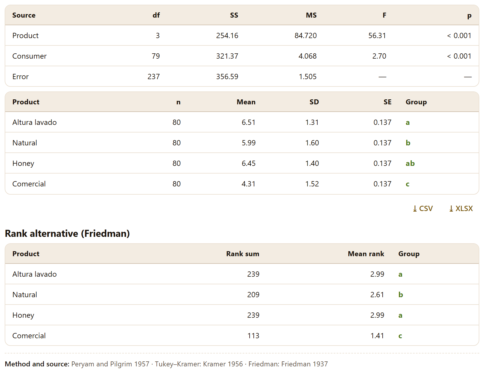
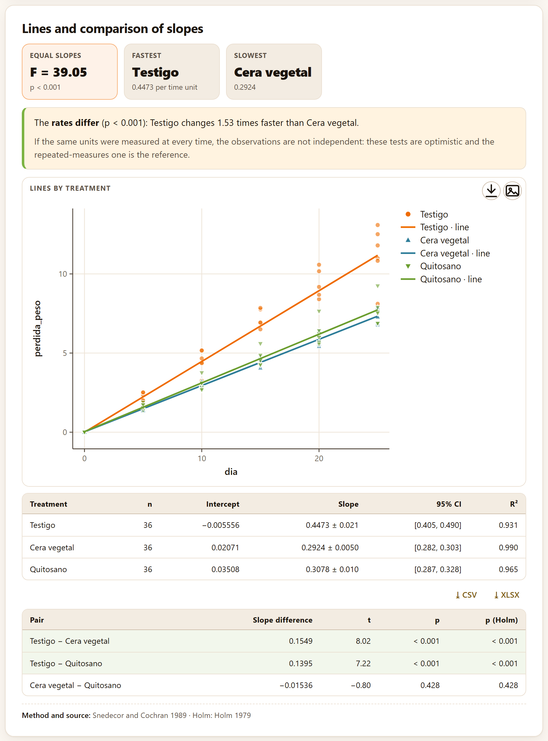
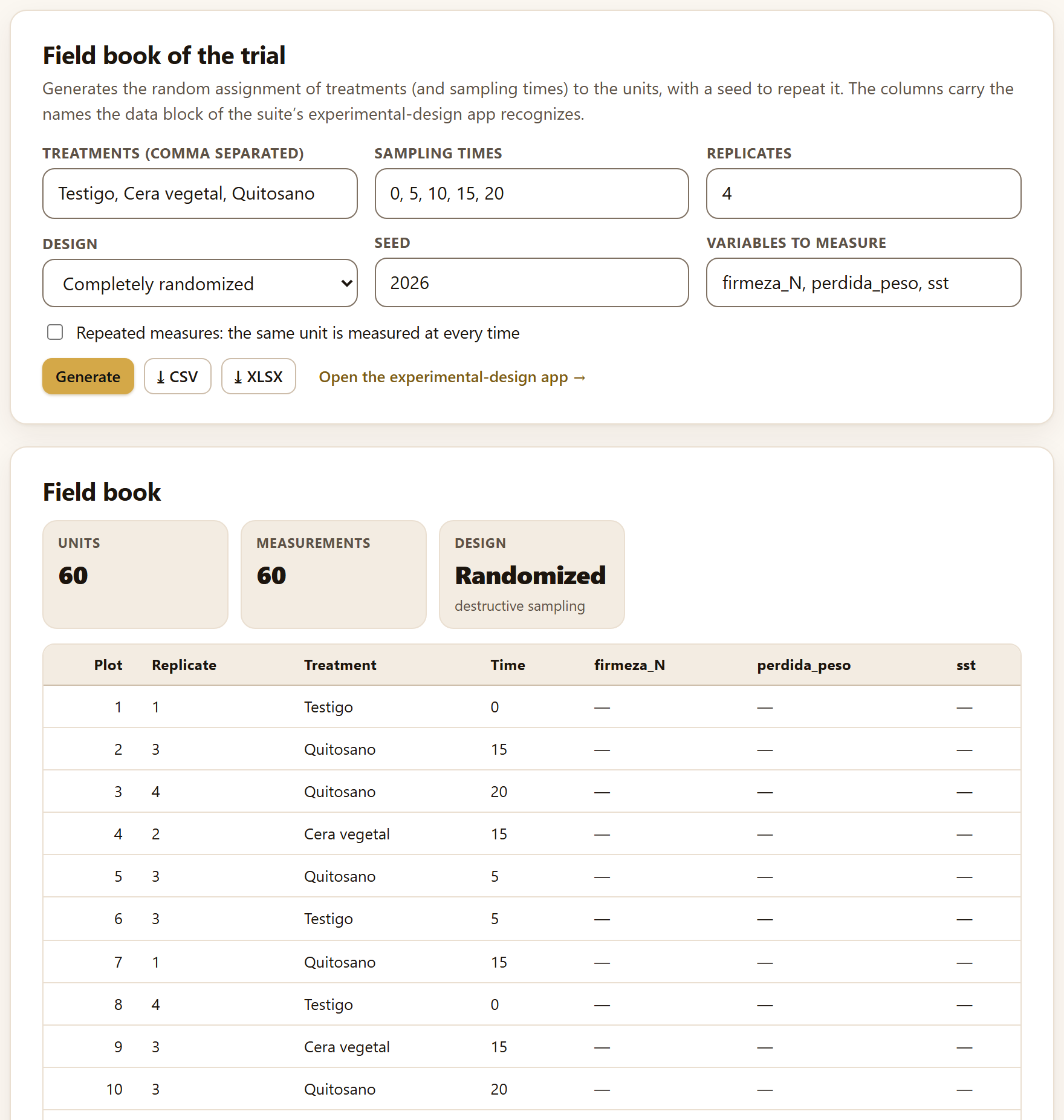
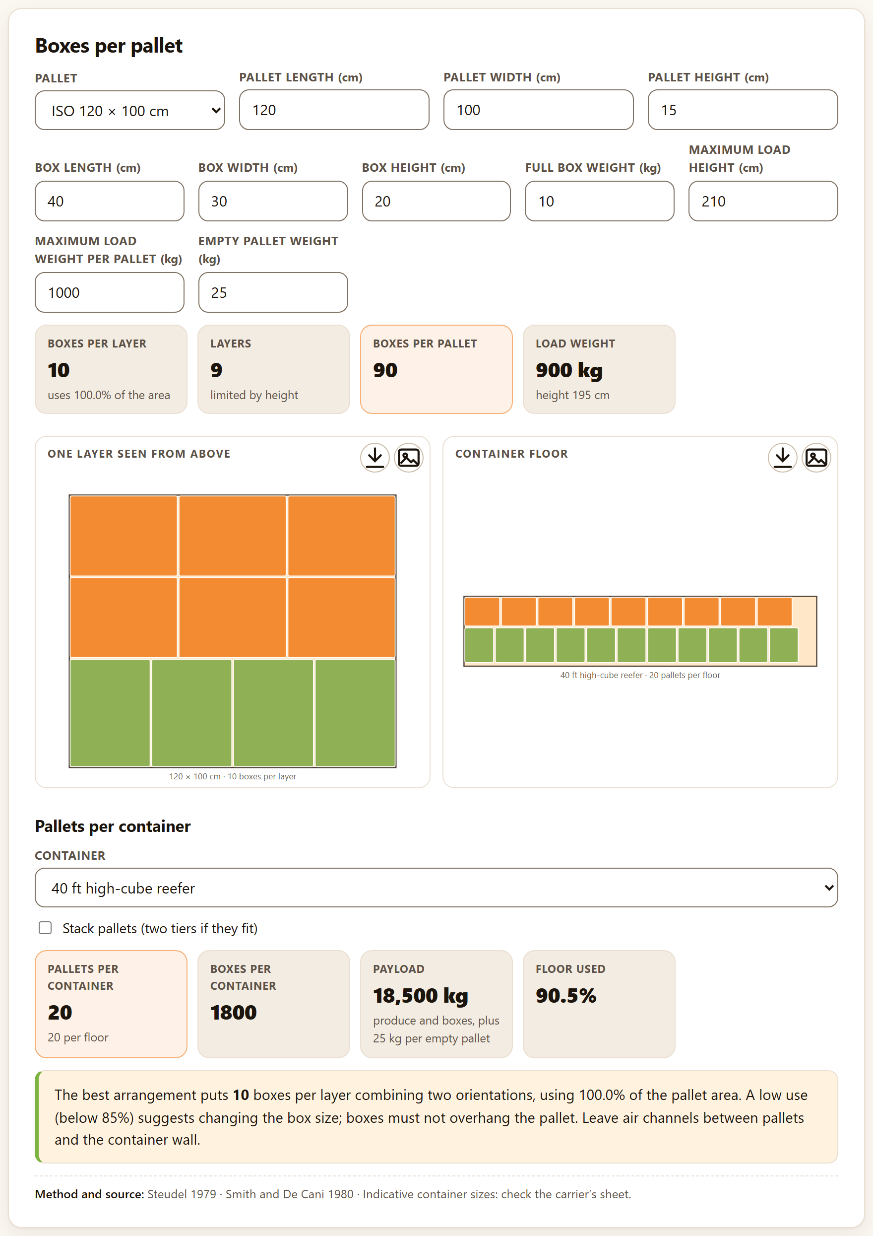
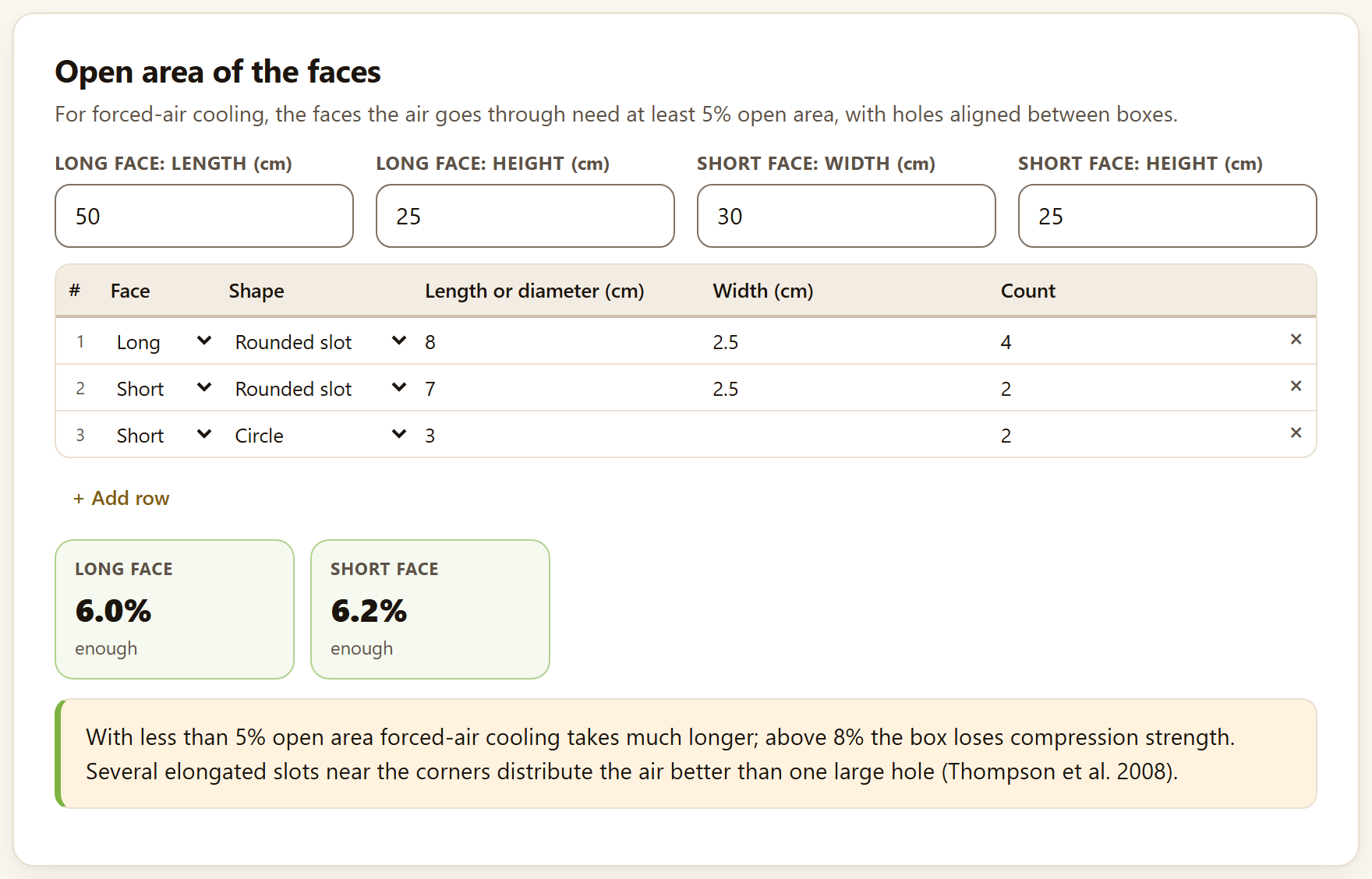
Spanish or English, with the ES · EN switch in the top bar. In this manual the names of buttons, fields and menus are written as they appear on screen in English, for example Take the k values to the temperature analysis →.
How to cite the program
Barrera-Guzmán, L. Á. (2026). PostHarvestPro: postharvest physiology and technology, quality, shelf life and sensory evaluation in the browser (Version 1.0.0) [Computer software]. Zenodo. https://doi.org/10.5281/zenodo.23935616
How to cite this manual
Barrera-Guzmán, L. Á. (2026). PostHarvestPro: User’s Manual (1st English ed.). Distributed with PostHarvestPro, version 1.0.0. https://doi.org/10.5281/zenodo.23935616
The program citation is the one the app itself gives, ready to copy, in the How to cite section of its home page and at the foot of Block 9. Both citations carry the Zenodo concept DOI, which always resolves to the latest version.
iPrivacy
PostHarvestPro runs entirely inside your browser. The tables you open or paste are read on your computer and are never sent to any server: you can work with the data of an ongoing trial, a company or a thesis without them leaving your machine. The program uses no accounts, loads nothing from the internet and needs no connection to compute.
The illustrations, diagrams and screenshots in this manual are original: they were generated with the program itself or with code written for the manual. Every figure comes from the app’s simulated example data—mango, chayote, avocado, tomato and coffee generated with models and parameters of the order of those published. They are not measurements of any real lot, orchard or panel.
The manual follows the order of the app: nine numbered blocks, listed from top to bottom in the bar on the left. Each chapter explains one block and carries its number—Chapter 4 is Block 4, with sections and figures 4.1, 4.2…. The introduction has no number: its sections are I.1, I.2….
Each chapter begins with what the block solves in postharvest handling, goes on with its tools in the order of their tabs and closes with the rules for reading the result and the most common mistakes. You need not read it from cover to cover: for the shelf life of a lot, Chapter 3 is enough; to design a package, Chapters 4 and 8; to prepare a tasting, Chapter 6. Appendix B gathers the rules and formulas of every block.
A color for each block
The color of a block appears on the opening page of its chapter, in each section number, on the tab at the page edge and in the contents, as in the strip on the cover. The app’s bar names some blocks with a short form (Shelf life, Losses, Sensory, Trials); the block title, above its tabs, gives the full name.
Block
Name in the app
What it does
1
Home
The work route, the nine blocks, the ten example data sets, the methods with their source, postharvest in plain words, the references and how to cite
2
Quality and maturity
Quality indices, CIELAB color, laboratory calculators, scales and size grades
3
Kinetics and shelf life
Reaction orders, temperature, accelerated tests and time to rejection
4
Respiration, ethylene and atmospheres
Respiration rates, climacteric, modified-atmosphere packaging and precooling
5
Losses and value chain
Quantity and value lost by stage, critical points, simulation and mechanical damage
6
Sensory evaluation
Discrimination, affective and descriptive tests, with the design of the tastings
7
Postharvest trials
Treatment × time factorials, repeated measures, slopes and randomization
8
Packaging and logistics
Loads, venting, cold-room environment, costs, compatibility and units
9
Report and project
Everything you computed in a document to share, and your work in a file to continue later
Types of boxes
iNote
Clarifications and practical tips that save time.
!Important
What can change your conclusions if overlooked.
θTheory in brief
The idea behind a computation, without unnecessary formulas.
▸Worked example
A case with the program’s example data, with the numbers the app gives.
✓Decision rule
If the result falls in this case…
then this is the recommended reading.
They are guides for interpretation, not laws: what you know about the crop, the cultivar and how the trial was run always prevails.
✕When something goes wrong
What usually fails in the block—a wrong column, a table in wide format, a temperature outside the measured range—and how to fix it.
10.7
Key figure
A number or fact worth remembering; for instance, the joules of heat a product releases per milligram of CO₂ it respires.
Writing conventions
Written like this
Means
Load example
A button, field or menu of the app, with its text exactly as it appears on screen in English.
Block 3›Temperature
A path: open the block and, inside it, the tab or card that follows.
Ctrl + K, mango_temperaturas.csv, firmeza_N
A key, a file or column name, or a value typed as is.
shelf life, limit
How long a product stays acceptable; the value of an attribute (25 N of firmness, say) beyond which it no longer is. Appendix C defines all terms.
k, Eₐ, Q10
The deterioration rate constant, the activation energy and the factor by which deterioration speeds up with 10 °C more (Chapter 3).
25.9 d · 59.4 mg CO₂ kg⁻¹ h⁻¹
Numbers have a decimal point, as in the app, and the unit separated by a space.
I
Introduction
Introduction to PostHarvestPro
Between harvest and the consumer, a fruit respires, loses water, softens, changes color and, sooner or later, is rejected. Measuring those changes is only half the job; the other half is turning them into decisions: how long a lot lasts, at what temperature to store it, what package to use, where most is lost and whether the consumer notices the difference. PostHarvestPro does that second half.
I.1What is PostHarvestPro?
I.2The questions it answers
I.3Six ideas that hold up the manual
I.4What data it accepts and what it delivers
I.5What you need and how to open it
I.6A tour of the interface
I.7The example data
I.8How a study is carried out
I.9How it was checked
I.10What the program does not do
I.1What is PostHarvestPro?
It is a postharvest physiology and technology program that runs in the browser, with nothing to install. It brings together in one place the computations that accompany a fruit or vegetable from harvest to the consumer, and it explains every result in words and says which method and which source it comes from.
It computes quality and maturity indices and color in CIELAB with its differences; it fits the kinetics of deterioration and predicts shelf life at one temperature or at any, including the time to rejection with fruit still sound when the trial ends; it measures respiration and ethylene, recognizes the climacteric and designs modified atmospheres, precooling and its heat load; it quantifies the losses of a chain in kilograms and in money, and mechanical damage; it analyzes discrimination, affective and descriptive sensory evaluation and designs the tastings; it analyzes postharvest trials with destructive sampling or with the same fruit over time; it solves the packaging, storage and transport calculations; and, at the end, it assembles a report with handling recommendations.
It is intended for teaching and research in postharvest, for quality control in packinghouses and marketers, and for anyone who advises growers. Everything is computed with engines written from scratch for this program, without other people’s libraries, and every method cites the work that defines it: on the app’s home page, at the foot of every result and in the methods of the report.
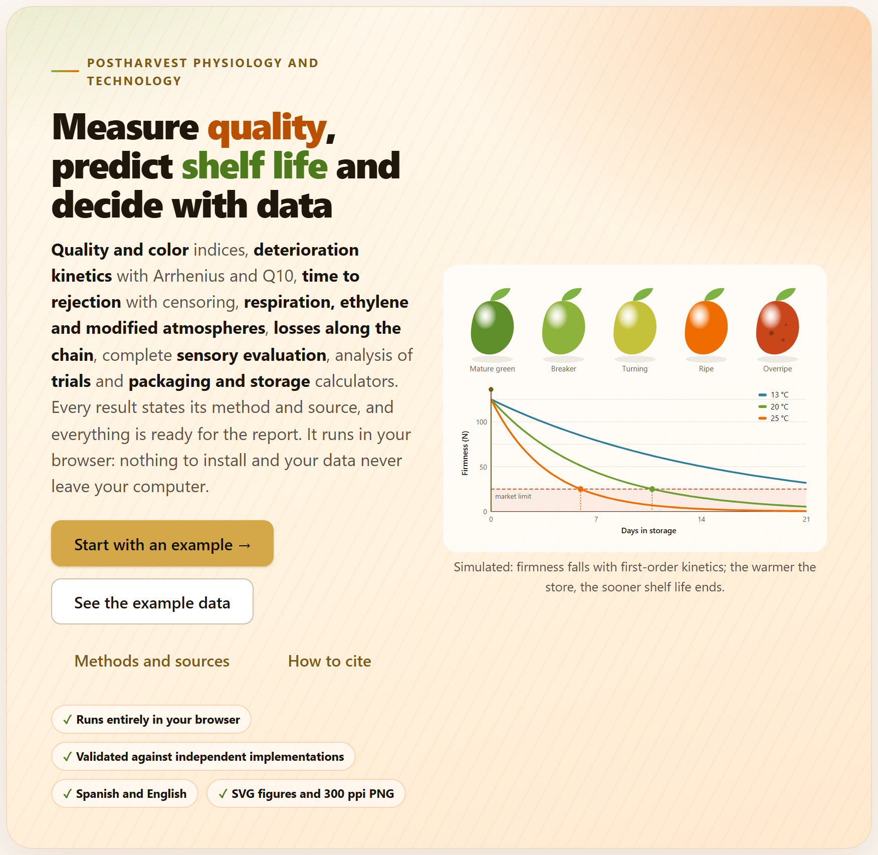
Figure I.1. The PostHarvestPro home page when it opens. On the left, the bar of the nine blocks; in the center, the motto, the buttons to get started and the illustration: a fruit in five stages of ripeness and the firmness of three lots stored at 13, 20 and 25 °C with their market limit; on the right, the sections of the home page.
I.2The questions it answers
A good way to find out whether the program is for you is to see which questions it answers, and in which block.
Question
Block
How do the firmness, soluble solids, acidity and color of each lot change over time? What is their SSC/TA?
2
How different are two colors, and what is the damage index or the marketable fruit of each lot?
2
With what reaction order is quality lost, and how many days does it take to reach the acceptable limit?
3
How long does the product last at 5 °C if I only measured it at 13, 20 and 25 °C? How much does each 10 °C speed up deterioration?
3
Which coating delays rejection most, counting the fruit still sound at the end?
3
How much does the product respire and how much heat does it release? Is it climacteric?
4
Which film and which thickness bring the package atmosphere into the recommended window? How long does it take to cool, and what equipment is needed?
4
At what stage of the chain are the most kilograms and the most money lost, and where does investment pay off best?
5
From what drop height is the fruit bruised?
5
Do the judges notice the difference, how many judges do I need, which product is liked most and which attribute penalizes it?
6
Do the treatments differ, at which times, and which one changes fastest?
7
How many boxes fit per pallet and per container? How much water does the product lose in the cold room? Can two products travel together?
8
How do I deliver the results, with their methods and some handling recommendations?
9
I.3Six ideas that hold up the manual
Everything that follows rests on six ideas. If you keep them in mind, many of the mistakes made when analyzing postharvest data are no longer possible.
Temperature rules. Almost all deterioration speeds up with temperature, and not in a straight line: with a typical activation energy, each extra 10 °C multiplies the rate by three or four. That is why Chapter 3 does not stop at “the lot lasted 10 days”: it takes the constants to Arrhenius and predicts the life at the storage temperature.
The reaction order is chosen on the original scale. Linearizing a curve and comparing R² values changes the scale of the error and misleads. The app fits the three orders by nonlinear least squares and compares them by their AIC.
A fruit still sound at the end is not lost data. If the trial ends before every fruit is rejected, the survivors are censored: they contribute information while they were under observation. Discarding them shortens the estimated life.
A loss is measured in kilograms and in money. What is lost at the start of the chain weighs more; what is lost at the end is worth more. The best investment is not always where the most kilograms are lost.
The unit of analysis is the one that was randomized. If different fruit are sampled each day, the trial is a factorial; if the same fruit are weighed every day, it is a repeated-measures trial and its p-values must be corrected. In a tasting, each consumer is a block.
A model summarizes what was measured; it does not replace it. Predictions outside the temperatures, times or cultivars measured are extrapolations, and the app says so when it happens. The tables of permeabilities, size grades and compatibility are a guide only: use those of your film, your standard and your cultivar.
I.4What data it accepts and what it delivers
Every tool that analyzes a table has the same data input: Load example, Open file (CSV, TXT, XLSX, ODS), Paste a table or dropping the file on the box. Then the app proposes which column plays each role—time, group, attribute, consumer, product…—by its name, and you confirm or change the proposal. The direct-computation tools (the laboratory calculators, temperature, modified atmosphere, all of Block 8) are filled in by typing in their fields or in editable tables, where + Add row adds a line and × removes it.
In
Format and where
Data tables
CSV, TSV or TXT separated by comma, semicolon or tab (with semicolon or tab the decimal comma is understood), and XLSX, XLSM or ODS workbooks; if the workbook has several sheets, a selector appears. Always in long format: one row per observed unit (fruit, jar, consumer per product) and one column per variable
Pasted cells
Copied from a spreadsheet, with the column names in the first row
Missing values
Empty cells, NA or — are taken as missing
Projects
A .json saved earlier by the app itself (Block 9)
Out
Format
Figures
Course of the attributes, color, kinetic curves, Arrhenius, Kaplan–Meier, respiration, O₂–CO₂ plane, Sankey, damage curves, psychometric curves, penalties, spider plots, maps, treatment profiles, pallet and psychrometric chart, among others: as SVG or as 300 ppi PNG, and in the suite’s figure studio
Tables
Every results table as CSV or XLSX, ready for a spreadsheet
Report
A single HTML file with cover, summary, one section per analysis with its figures, tables and interpretation, handling recommendations, methods, references and citation; it prints to PDF from the browser
Work plans
The serving plan of a tasting (CSV) with its ballots for printing, and the randomized field book of a trial (CSV or XLSX)
For other apps
The loss chain for EconomicsPro, the means of a descriptive profile for PCAPro and the field book for AgriDesign, from the same suite
I.5What you need and how to open it
Only a modern browser, in a version from the last few years, on a computer, a tablet or a phone. There is nothing to install and no internet is needed; the whole program fits in one folder.
Double-click index.html. It is the simplest way and everything works the same: the computations and the ten example data sets are inside the program.
Or double-click Open PostHarvestPro.bat. It starts a minimal local server on port 9970 and opens the app at http://localhost:9970. You only need it to open the app from another computer or a tablet on the same network; the server.ps1 file explains how.
Or online, at the app’s address in the LABG Suite, once it is published.
Your preferences—the language, the light or dark theme and the last tab you opened in each block—are kept in the browser itself and remembered next time. The data are not: every time you open the app it starts empty. To resume a piece of work there is the .json project of Block 9, which saves the tables you loaded, the columns you chose, the edited tables and the settings, and recomputes everything when you open it. If you try to close the tab after having worked, the app warns you.
This manual opens from the app itself: the User’s manual link is at the foot of its home page (Block 1); with the interface in Spanish, the link leads to the Spanish edition.
I.6A tour of the interface
All the applications of the suite share the same bar, the same navigation and the same figure tools, so what you learn here also serves you in the others.
123456789101112
Figure I.2.Block 3›Kinetic models with the example mango just loaded. The numbers refer to the list below.
1Name of the app and its motto. The name leads to the home page (Block 1).
2LABG Suite. Goes back to the portal with the other applications.
3ES · EN. Changes the language of the whole interface, including that of the figures and of the report.
4Theme, animations, report and help. The sun switches between the light and the dark theme; the sparkles button turns animations off or on; the speech bubble opens “Report a problem”; the question mark, the list of shortcuts (key ?).
5The bar of the nine blocks. The number turns into a check mark when the block already has a result, and the count at the top says how many there are (1/9 in the figure).
6The path. The app, the block, the tab and the card you are in.
7Document · Focused. All the cards of the block one after another, or one at a time; the button next to it collapses or expands them all.
8Search (Ctrl + K). A block, a section, a control or a figure, by its name.
9In this block. The tabs of the open block and, inside the current one, its cards; the one you are viewing is highlighted.
10The block title, with its number and what it does in one line.
11The tabs. Each block divides its tools into tabs; the app remembers the last one you opened in each.
12The data input. The example data set with its description and its SIMULATED tag, the buttons to load it or open your file and, below, the column for each role.
Getting around without getting lost
At the foot of each block two buttons lead to the previous and the next one. When you change a control and the results are recomputed further down, a floating button appears that takes you back to the control you touched, and another to go back to the top. Results are redone by themselves: when you change a setting, instantly; when you load new data—an example, a file, a pasted table or another column—the analysis runs inside the suite’s waiting screen, which only appears, with the message Analyzing the data…, if it takes more than a moment. Almost everything can also be done from the keyboard:
Key
What it does
Alt + ← · Alt + →
The previous or the next block; in focused mode, the previous or the next card
Ctrl + K
Search for a block, a section, a control or a figure
[
Collapse or open the bar of the blocks
← · → on the tabs
The previous or the next tab of the block
?
Show the list of shortcuts
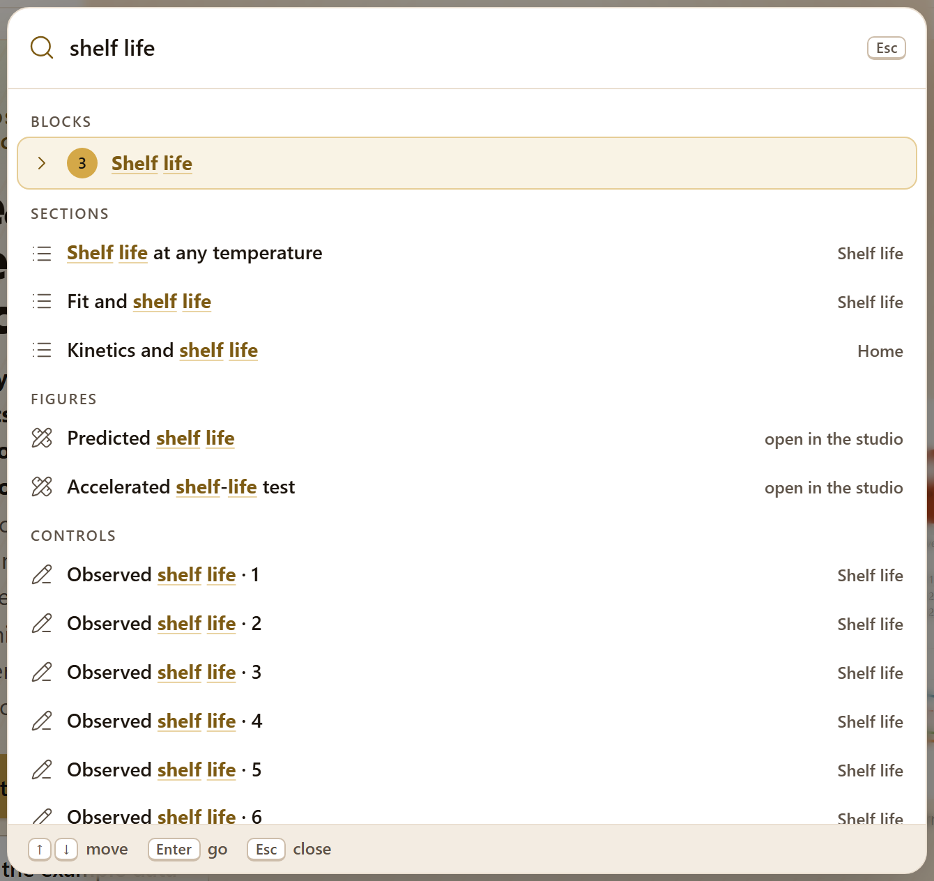
Figure I.3. The search (Ctrl + K) with “shelf life” typed: it finds Block 3, the cards that deal with shelf life, two figures—which open in the figure studio—and the fields of the accelerated test. Enter goes to the chosen result.
Every result is explained
Below each analysis there are three things besides the figures and the tables: some tiles with the numbers that matter (the chosen order, the life to the limit, the p-value), a reading in words of what they mean for the product, and the line Method and source: with the method and the citation. When something calls for care—an extrapolation, a straight line with a low R², a time that not all treatments have—a warning says so in the same place.
The figures
Every figure in the app can be opened in the figure studio, a window shared by the whole suite where you change the texts, the font size, the legend and the colors without touching the data, and export to PNG, SVG, PDF or TIFF at 300, 600 or 1200 ppi. Next to each figure, the ✎ button opens the figure editor, and two quick buttons download it as SVG or as a 170 mm PNG at 300 ppi. Downloads and the report always use the colors of the light theme, even if you are working in the dark one. Chapter 9 explains this in depth.
I.7The example data
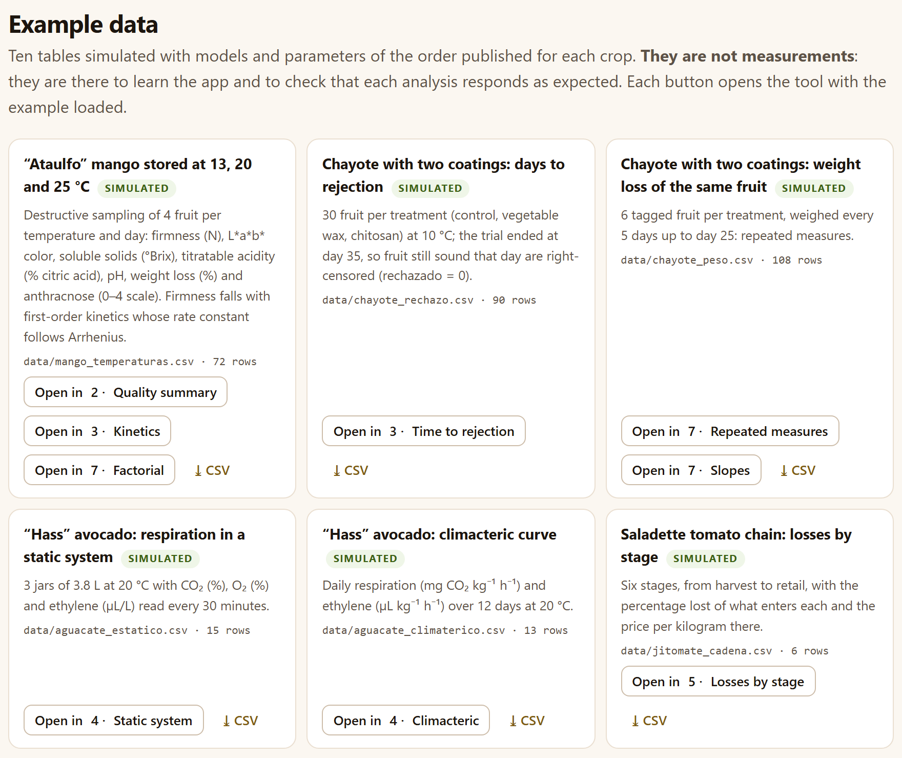
So that you can learn without data of your own, the app comes with ten simulated tables: they were generated with models and parameters of the order of those published for each crop, with a fixed seed, so they are always the same. They are not measurements: they are there to learn the app and to see that each analysis responds as expected. Each tool offers them with Load example and marks them with the SIMULATED tag, and the Example data section of the home page gathers them, with a button to open each tool with its example loaded and another to download the CSV.
Figure I.4.Block 1›Example data: the first six of the ten simulated tables, with the file in data/ they come from, their number of rows and the Open in … buttons that take you to each tool with the example loaded.
The ten example data sets, all simulated
File
Content
Rows
Blocks
mango_temperaturas.csv
“Ataulfo” mango at 13, 20 and 25 °C; 4 fruit per temperature and day: firmness, L*a*b*, soluble solids, acidity, pH, weight loss and anthracnose
72
237
chayote_rechazo.csv
Chayote with control, vegetable wax and chitosan at 10 °C, 30 fruit each: days to rejection; the trial ended at day 35
90
3
chayote_peso.csv
The same treatments: 6 tagged fruit per treatment, weighed every 5 days up to day 25
108
7
aguacate_estatico.csv
“Hass” avocado in 3 jars of 3.8 L at 20 °C: CO₂, O₂ and ethylene every 30 minutes
15
4
aguacate_climaterico.csv
Daily respiration and ethylene over 12 days at 20 °C
13
4
jitomate_cadena.csv
Six stages of a saladette tomato chain, from harvest to retail: loss and price
6
5
jitomate_caidas.csv
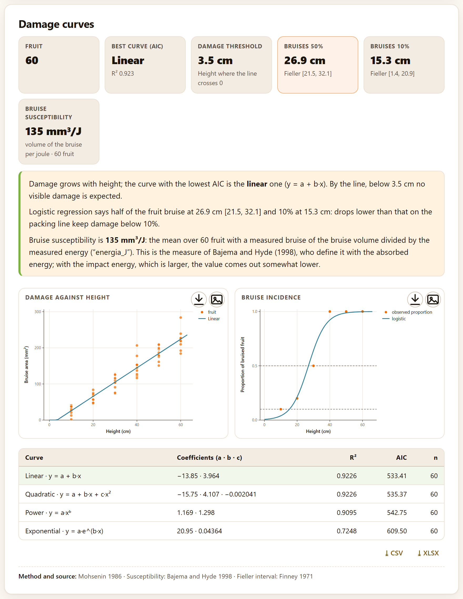
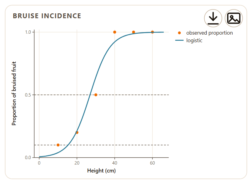
10 fruit per drop height, from 10 to 60 cm: mass, energy, bruise area and volume, and whether it was bruised
60
5
cafe_discriminativas.csv
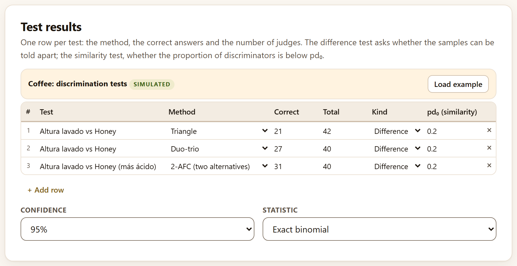
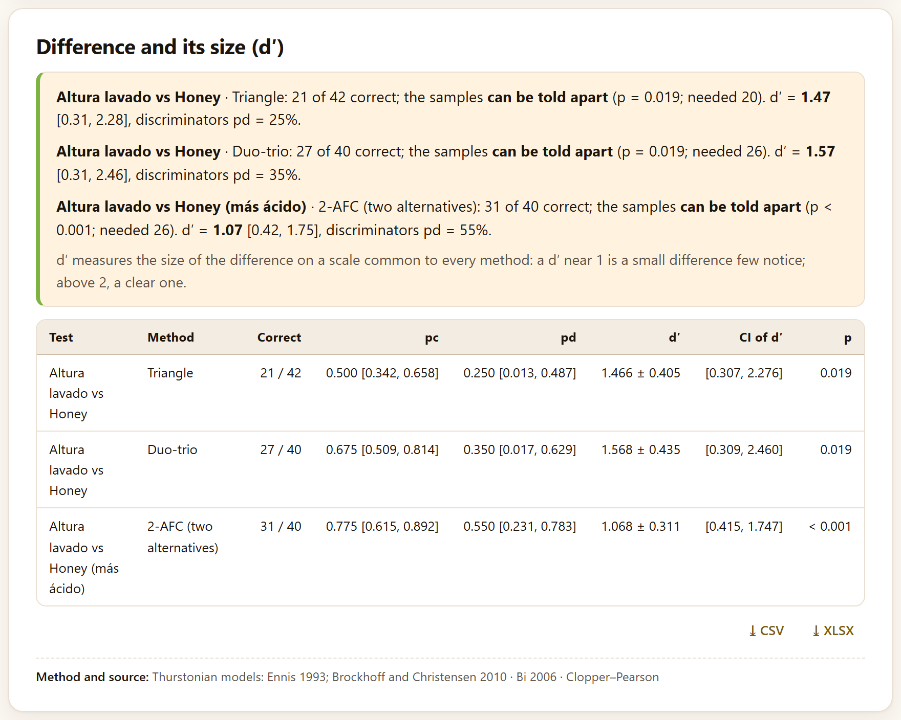
Triangle, duo-trio and 2-AFC between two coffees: correct answers and judges
3
6
cafe_consumidores.csv
80 consumers × 4 coffees: 9-point liking, just-about-right for acidity, bitterness and body, and 10 CATA terms
320
6
cafe_descriptivo.csv
8 judges × 4 coffees × 2 sessions, 7 attributes from 0 to 10
64
6
The tools that do not read a table—the calculators, temperature, the accelerated test, flow-through, modified atmosphere, precooling, the simulation of improvements, the ballots, randomization and all of Block 8—open with example values already typed in their fields, so that the result shows from the start.
▸The thread of the manual: the mango
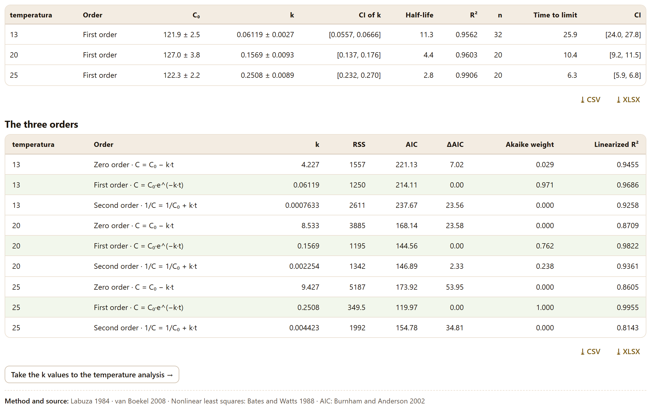
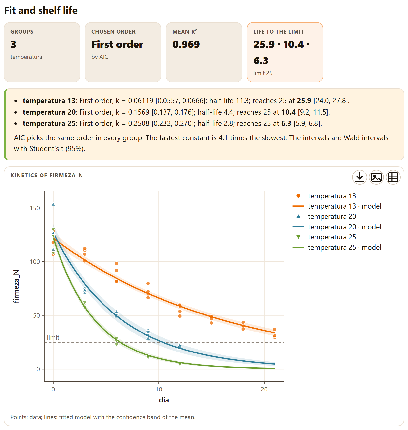
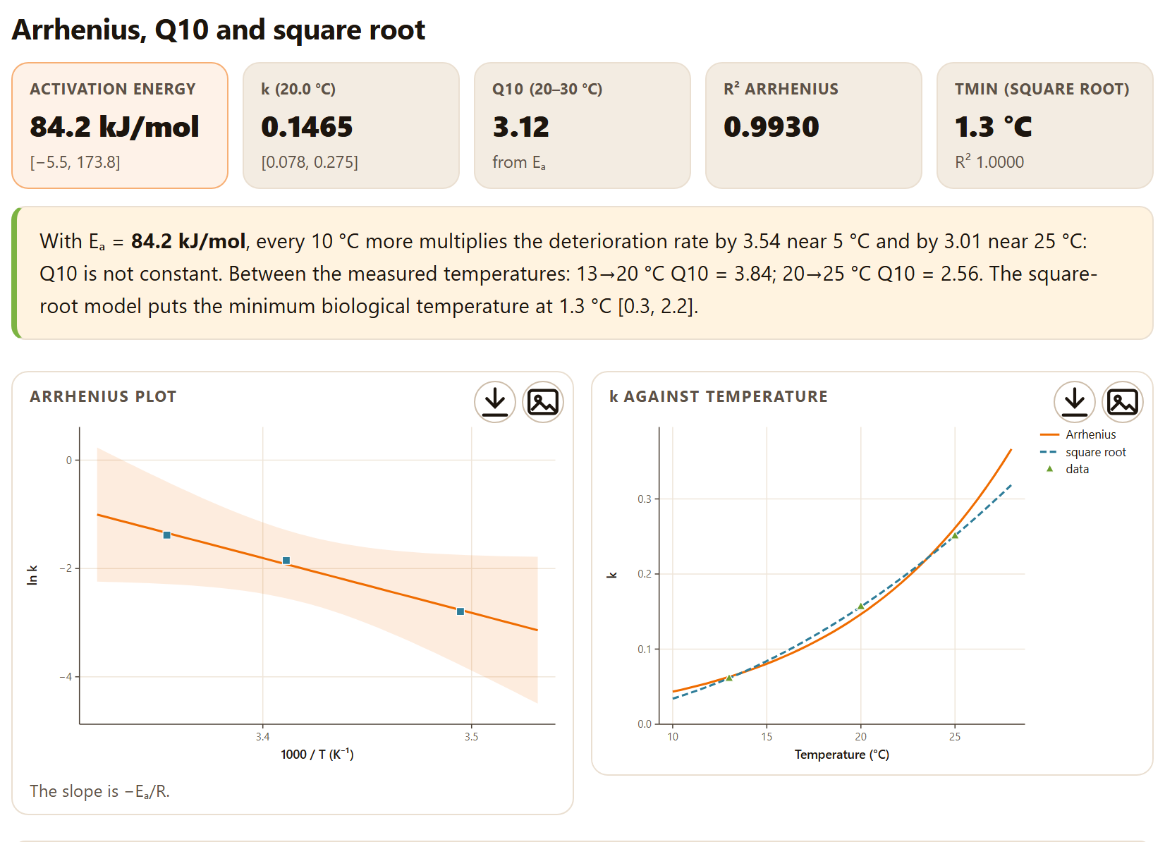
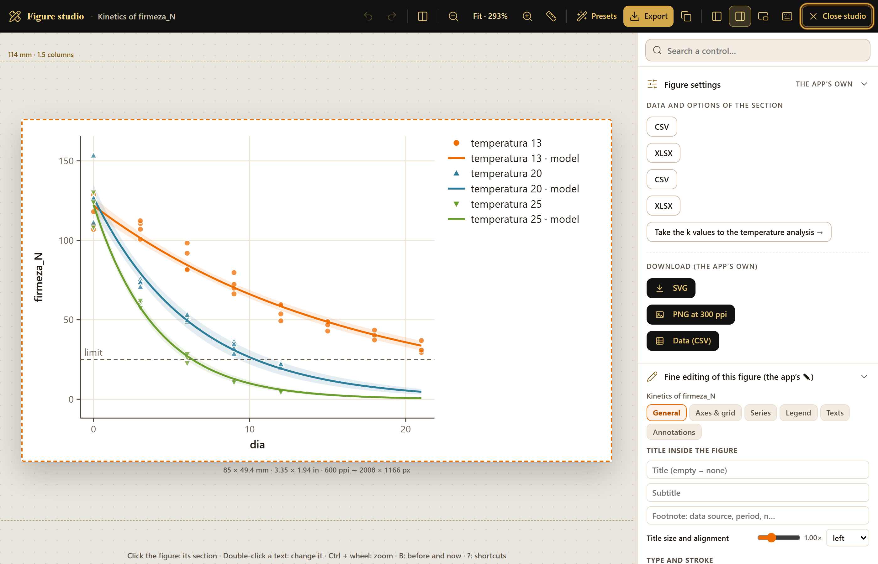
The firmness of the example mango falls from about 116 N to 32 N in 21 days at 13 °C, and from 122 N to less than 5 N in 12 days at 25 °C. In Block 3 the app chooses the first order at all three temperatures, with k = 0.0612, 0.1569 and 0.2508 per day, and computes that firmness reaches the 25 N limit at 25.9, 10.4 and 6.3 days. With those three constants, Arrhenius gives an activation energy of about 84 kJ/mol. It is the example drawn on the cover of this manual.
iThe whole manual comes from these examples
Every screenshot and every number in this manual comes from the simulated example data, with the default value of each control unless the text says what was changed. The text says “the example mango,” never as if it were a real lot.
I.8How a study is carried out
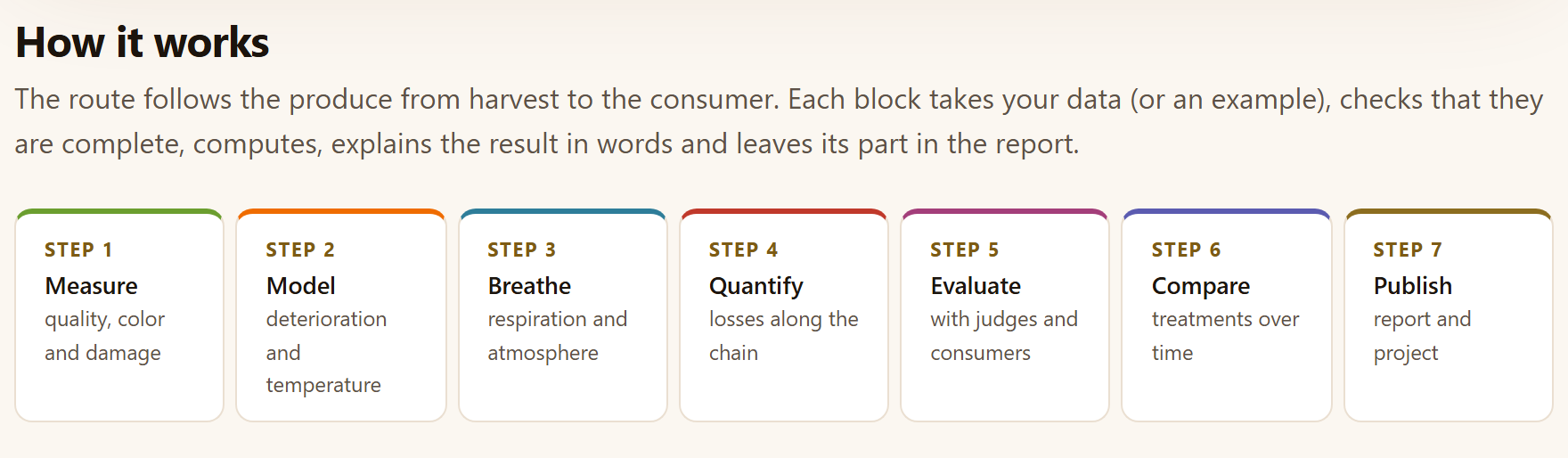
The blocks follow the product from harvest to the consumer. You do not need to go through all of them, nor in order: each tab works with its own data, and whatever you compute leaves its section in the report. The How it works section of the home page sums up the route in seven steps.
Figure I.5.How it works: the seven steps of the route, from measurement to the report.
Measure (Block 2). Summarizes the quality of each lot over time, converts and compares colors, computes acidity, moisture and firmness, and turns damage scales and size grades into indices.
Model (Block 3). Fits the kinetics of an attribute, takes its constants to temperature and predicts shelf life; or, if what you have is the day each fruit was rejected, estimates the survival curves.
Breathe (Block 4). Measures respiration and ethylene, recognizes the climacteric and designs the package, precooling and refrigeration.
Quantify (Block 5). The losses of the chain in kilograms and in money, where improving pays off and from what height the fruit is bruised.
Evaluate (Block 6). With judges and consumers: whether the difference is noticed, how much it is liked, what penalizes it and how a panel describes it.
Compare (Block 7). The treatments of a trial throughout storage, with the analysis that matches how it was sampled. Block 8 adds the packaging, storage and transport calculations.
Publish (Block 9). The report with all of the above and the handling recommendations, and the project to continue another day.
iSome results pass from one tab to another
Take the k values to the temperature analysis → copies the constants of the kinetic models to the Temperature tab when the group is the temperature; the Simulate improvements tab works on the chain of Losses by stage; and Block 9 gathers the sections of the tools you used in the others. The check mark of a block in the bar lights up when it already has a result.
I.9How it was checked
A computing program is worth what its numbers are worth. Every engine in PostHarvestPro was programmed from the published formula and compared, number by number, with an independent implementation: the R statistical environment (version 4.4.2) and its reference packages for nonlinear kinetics, survival analysis, sensory evaluation and trial analysis; published tables for color and psychrometrics; and hand computations written into the tests themselves for the calculators. Every comparison has its tolerance written down.
71,283
Comparisons without failures
In 450 automated tests, which run in the browser by double-clicking tests/run.html and in the console with node tests/run-node.js. The table below breaks them down by engine.
Validation by area (node tests/run-node.js; the details, in tests/validacion/)
Area
Tests
Comparisons
Reference
Numerical core
6
534
Distributions, regression, eigenvalues, nonlinear fitting and p-value adjustment in R
Color
6
1,115
Conversions and ΔE from an R color package; the 22 published pairs of Sharma, Wu and Dalal (2005); the whiteness, yellowness and tomato indices by hand
References
2
96
That every source in the list of methods is in the list of references
Quality
4
28
Hand computations (acidity, moisture, McKinney, size grades)
Respiration and atmospheres
3
19
Hand computations (gas balances, steady state, cooling)
Losses and damage
3
45
Linear and logistic regression in R and Fieller interval
Logistics
3
36
ASHRAE (2017) saturation tables and psychrometric identities
Kinetics
233
18,932
R nonlinear least squares with two algorithms, and linear regression
Time to failure
143
38,488
Kaplan–Meier, log-rank and parametric models from two R survival packages
Sensory
32
11,669
R packages for sensory analysis, factor analysis and multiple comparisons
Trials
8
242
Type I and III analysis of variance, Tukey, Dunnett, repeated measures with Mauchly and comparison of slopes in R
Figures
7
79
Geometry and text written into the test: thousands on the axes, labels that do not overlap, distinct strokes and the percent sign of each language
Total
450
71,283
0 failures
The comparison also served to correct. It caught, among others, a cutoff in the studentized range that set probabilities to zero with five or more means, standard errors of the logistic regression computed with the weights of the next-to-last iteration and an optimizer that declared convergence next to the pole of a second-order curve; all three were corrected before version 1.0. The details, with the tolerances of each test, are in the tests/validacion/ folder, which is the only part of the program that names software packages: the app and the rest of this manual describe the methods and cite the articles.
I.10What the program does not do
Knowing where a tool ends is as useful as knowing what it does. The app’s home page says so in What it does not do, and the chapters repeat it where it matters:
It does not
Why, and what to do
Replace measurement
The models summarize the data; extrapolating far from the temperatures, times or cultivars measured is your responsibility, and the app warns when it happens.
Bring trade standards
The tables of size grades, film permeabilities, atmosphere windows and compatibility are a guide only and can be edited: use those of your standard, your film and your cultivar.
Model non-isothermal kinetics
Predictions are at constant temperature; for a variable temperature history, k(T(t)) has to be integrated over time.
Simulate package dynamics
The modified atmosphere is computed at steady state, with an unperforated film and a perfect seal; not the time it takes to get there.
Read instruments
It does not connect to texture analyzers, colorimeters or chromatographs: it works with the tables they export.
Upload your data
There is no server, no accounts and no connection: what you save is a project file on your computer.
1
Chapter one · Block 1
Home: the route, the examples and the methods
Block 1 is the app’s home page. It computes nothing: on a single screen it says what PostHarvestPro does, sums up the route of a product from harvest to the consumer, presents the eight working blocks, opens the ten example data sets in the tool that matches each one, lists the methods with their source, explains in plain words the physiology behind the computations and gives the program’s citation. It is the place you come back to when starting something new or to remember where everything is.
1.1The home page
1.2How it works: the route in seven steps
1.3The nine blocks
1.4Example data
1.5Methods and sources
1.6Postharvest in brief
1.7What it does not do
1.8References and how to cite
1.1The home page
When you open index.html, the app starts in Block 1. Unlike the other blocks, this one has no tabs and no data cards: it is a presentation page that you scroll from top to bottom, and the In this block list on the right leads to each of its sections.
At the top is the presentation panel. A small label states the subject of the app, Postharvest physiology and technology; below it comes the motto, Measure quality, predict shelf life and decide with data, and a paragraph that lists what it does, from quality indices and color to the packaging and storage calculators, and ends with two promises: every result states its method and its source, and the data never leave your computer.
123456
Figure 1.1. The presentation panel of the home page. The numbers refer to the list below.
1Start with an example → Opens Block 2›Quality summary and loads the example mango into it: the fastest way to see the app with data (Chapter 2).
2See the example data. Scrolls down to the Example data section of the same page (Section 1.4).
3Methods and sources. Scrolls down to the list of methods with their citation (Section 1.5).
4How to cite. Scrolls down to the program’s citation, at the end of the home page (Section 1.8).
5The four badges.Runs entirely in your browser, Validated against independent implementations, Spanish and English and SVG figures and 300 ppi PNG. They are only labels; they cannot be clicked.
6The illustration. A fruit in five stages of ripeness—Mature green, Breaker, Turning, Ripe and Overripe—over the firmness of three lots stored at 13, 20 and 25 °C, with the band of the market limit and the day the 20 and 25 °C curves cross it.
The illustration has its caption: Simulated: firmness falls with first-order kinetics; the warmer the store, the sooner shelf life ends. It is a drawing, not a result: it does not change with the data you load. But it sums up the central idea of the program, the one Chapter 3 turns into numbers: the same fruit, with the same initial firmness, reaches the limit on very different days depending on the temperature at which it is stored. The curves are drawn from left to right when the home page opens; if you turn animations off with the sparkles button in the top bar, or if your system asks for reduced motion, they appear already drawn.
The three buttons below only scroll the page. The first one, on the other hand, does the same as the Open in 2 · Quality summary button on the mango card in Example data: it changes block and tab, loads the table and shows the results.
iThe home page is never cleared
Loading an example or your own data changes nothing in Block 1. What does change is the bar on the left: the number of a block turns into a check mark when that block already has a result. The PostHarvestPro name in the top bar always brings you back here.
1.2How it works: the route in seven steps
The first section below the presentation, How it works, sums up the route in seven numbered boxes (Figure I.5 of the introduction). Its subtitle explains it: The route follows the produce from harvest to the consumer. Each block takes your data (or an example), checks that they are complete, computes, explains the result in words and leaves its part in the report.
Table 1.1. The seven steps of How it works and the block that carries out each one
Step
Name
What the app says
Where it is done
1
Measure
quality, color and damage
2 Quality and maturity (Chapter 2)
2
Model
deterioration and temperature
3 Kinetics and shelf life
3
Breathe
respiration and atmosphere
4 Respiration, ethylene and atmospheres
4
Quantify
losses along the chain
5 Losses and value chain
5
Evaluate
with judges and consumers
6 Sensory evaluation
6
Compare
treatments over time
7 Postharvest trials
7
Publish
report and project
9 Report and project (Chapter 9)
Block 8, Packaging and logistics, has no step of its own: its pallet, venting, storage and compatibility calculations go along with any of the steps, as Section I.8 says. The route is there so that you forget nothing, not to impose an order: each tab works with its own table, and you can go straight to Block 6 to analyze a tasting without having gone through the others.
1.3The nine blocks
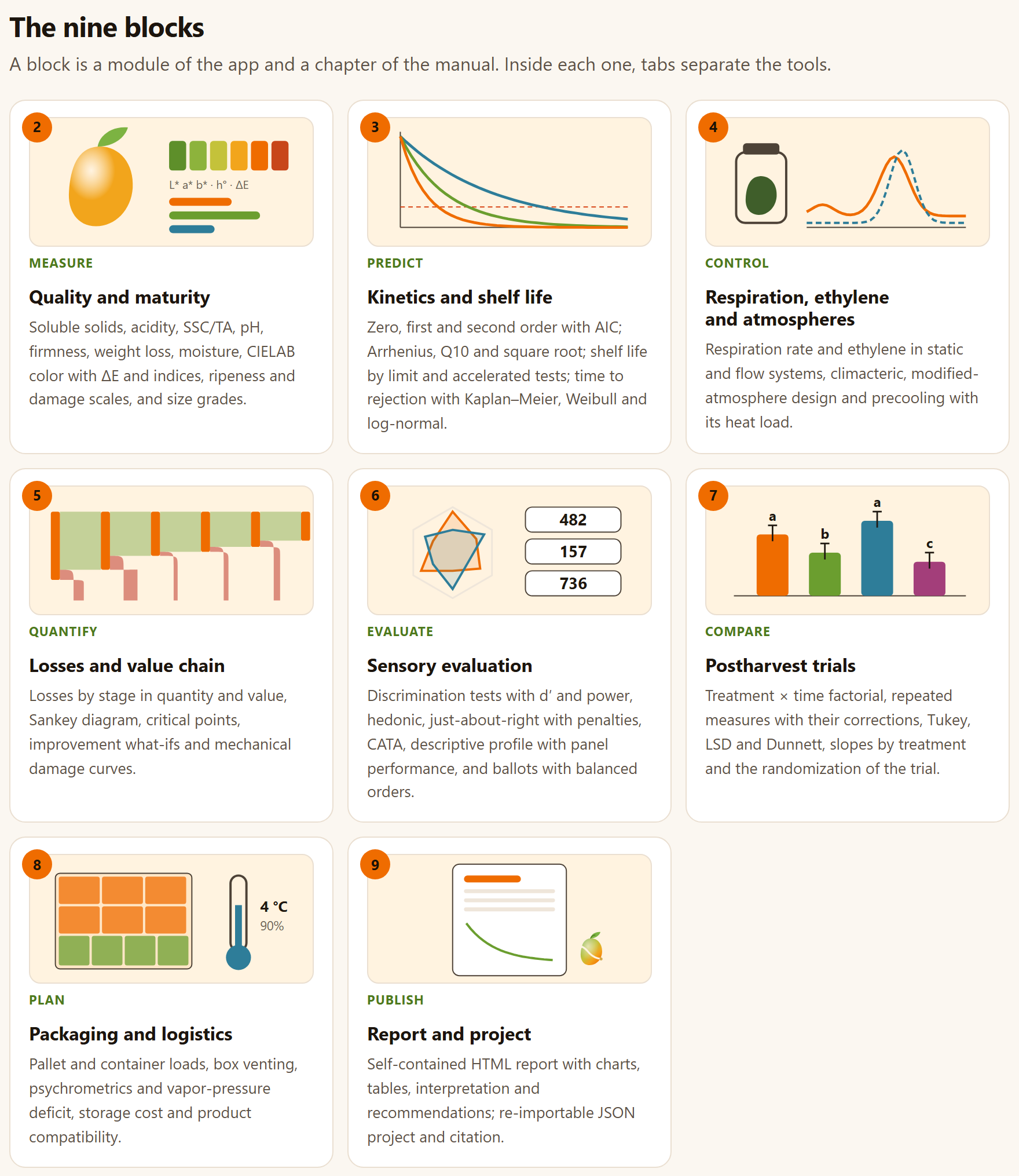
The The nine blocks section has one card for each block from 2 to 9 (Block 1 is this very home page). Each one carries the block number, a drawing of its own made by code, a tag with the verb of what it does, the name of the block and the same line the app puts below its title. A click anywhere on the card opens the block. The subtitle of the section sums up the correspondence with this manual: A block is a module of the app and a chapter of the manual. Inside each one, tabs separate the tools.
Figure 1.2.The nine blocks. The drawings sum up each block: a mango next to its color scale and the line L* a* b* · h° · ΔE (2), three deterioration curves crossing a limit (3), a respiration jar next to a climacteric peak (4), a chain that loses produce at each stage (5), a spider plot and three sample codes (6), bars with their comparison letters (7), a pallet and a thermometer at 4 °C and 90% (8) and a report sheet (9).
Table 1.2. The tags of the cards and the chapter of each block
Block
Tag
Name
Chapter
2
Measure
Quality and maturity
2
3
Predict
Kinetics and shelf life
3
4
Control
Respiration, ethylene and atmospheres
4
5
Quantify
Losses and value chain
5
6
Evaluate
Sensory evaluation
6
7
Compare
Postharvest trials
7
8
Plan
Packaging and logistics
8
9
Publish
Report and project
9
At the foot of the home page, as at the foot of every block, a button leads to the next one: Next · 2 · Quality and maturity →. From the keyboard, Alt + → does the same.
1.4Example data
The Example data section gathers the ten simulated tables that come with the app, one per card (Figure I.4 of the introduction). Its subtitle gives the warning: Ten tables simulated with models and parameters of the order published for each crop. They are not measurements: they are there to learn the app and to check that each analysis responds as expected. Each button opens the tool with the example loaded.
Each card has the name of the data set with the SIMULATED tag, a description, the file in data/ it comes from with its number of rows, one Open in … button for each tool that uses it and the ⤓ CSV button, which downloads the table so that you can see its layout or use it as a template for yours. The table in Section I.7 says what each data set contains; the one below, where each button leads.
Table 1.3. The Open in … buttons of Example data
Card
Buttons
“Ataulfo” mango stored at 13, 20 and 25 °C · 72 rows
Open in 2 · Quality summary, Open in 3 · Kinetics, Open in 7 · Factorial
Chayote with two coatings: days to rejection · 90
Open in 3 · Time to rejection
Chayote with two coatings: weight loss of the same fruit · 108
Open in 7 · Repeated measures, Open in 7 · Slopes
“Hass” avocado: respiration in a static system · 15
Open in 4 · Static system
“Hass” avocado: climacteric curve · 13
Open in 4 · Climacteric
Saladette tomato chain: losses by stage · 6
Open in 5 · Losses by stage
Tomato: drop test (mechanical damage) · 60
Open in 5 · Mechanical damage
Coffee: discrimination tests · 3
Open in 6 · Discrimination
Coffee: 80 consumers (liking, just-about-right and CATA) · 320
Open in 6 · Hedonic, Open in 6 · JAR, Open in 6 · CATA
Coffee: quantitative descriptive profile · 64
Open in 6 · Descriptive profile
The mango also appears, without a button on the home page, in the Color, Ripeness and damage scales and Size grades tabs of Block 2, whose Load example button opens it right there. Each Open in … button does two things: it opens the tab and presses its Load example for you, which replaces whatever table that tool had.
!Examples replace what you have
Opening an example replaces the table of the tool that receives it. If you had already loaded your own data into it, save the project first (Block 9›Project, Section 9.6) so that you can go back to them.
1.5Methods and sources
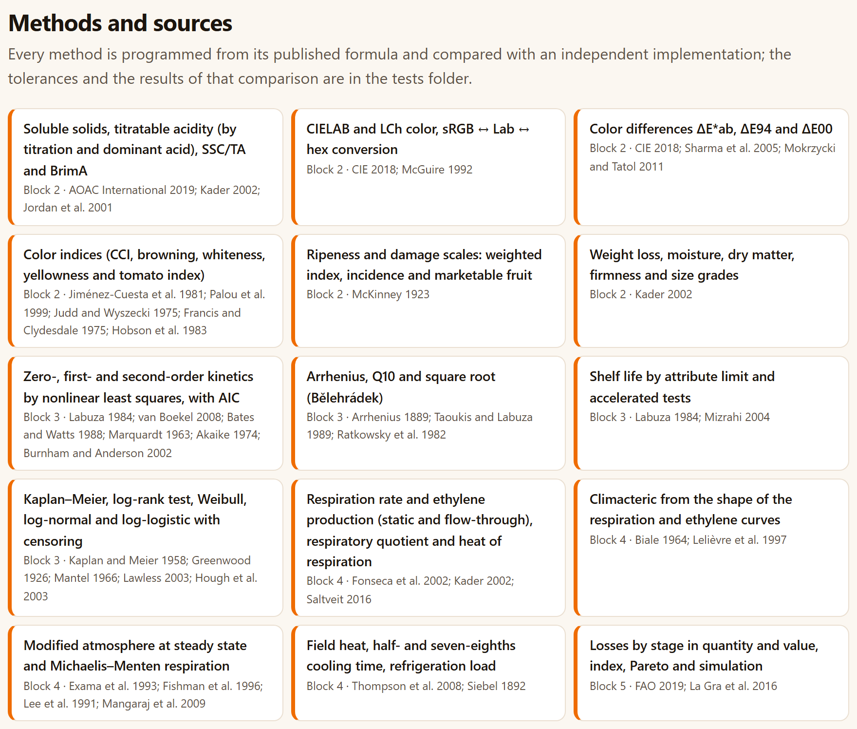
The Methods and sources section lists the program’s 28 methods, each on a card with its name, the block where it is used and the works that define it, abbreviated by author and year. The subtitle sums up how they were programmed: Every method is programmed from its published formula and compared with an independent implementation; the tolerances and the results of that comparison are in the tests folder.
Table 1.4. The thirteen cards that follow, from Blocks 5 to 8
Block
Method
Sources
5
Mechanical damage: impact curves, threshold, susceptibility and logistic regression with Fieller interval
Bajema and Hyde 1998; Mohsenin 1986; Finney 1971
6
Discrimination tests with Thurstonian d′, power and sample size
Ennis 1993; Ennis and Jesionka 2011; Brockhoff and Christensen 2010; Bi 2006; Clopper and Pearson 1934
Hedonic scale, ANOVA and Tukey; Friedman ranking
Peryam and Pilgrim 1957; Friedman 1937; Lawless and Heymann 2010
Just-about-right (JAR) with penalty analysis
Xiong and Meullenet 2006; Lawless and Heymann 2010
CATA: Cochran’s Q, McNemar and correspondence analysis
Meyners et al. 2013; Cochran 1950; McNemar 1947; Greenacre 2007
Descriptive profile: judge × product ANOVA, panel performance and PCA
Stone et al. 1974; Næs et al. 2010; Jolliffe 2002
Williams presentation orders and three-digit codes
Williams 1949; MacFie et al. 1989
7
Treatment × time factorial ANOVA (types I and III) and mean comparison
Steel et al. 1997; Kramer 1956; Dunnett 1955; Copenhaver and Holland 1988; Piepho 2004
Repeated measures: split plot in time, Greenhouse–Geisser, Huynh–Feldt, Mauchly
Steel et al. 1997; Greenhouse and Geisser 1959; Huynh and Feldt 1976; Lecoutre 1991; Mauchly 1940; Satterthwaite 1946
Comparison of slopes (analysis of covariance)
Snedecor and Cochran 1989; Holm 1979
8
Pallet and container loading patterns
Steudel 1979; Smith and De Cani 1980
Psychrometrics, vapor-pressure deficit and transpiration
ASHRAE 2017; Wagner and Pruss 2002; Wagner et al. 2011; Sastry et al. 1978
Box venting and storage compatibility of products
Thompson et al. 2008; Kader 2002; Gross et al. 2016; McGregor 1989
Figure 1.3.Methods and sources: the first fifteen cards, with the six methods of Block 2, the four of Block 3, the four of Block 4 and the first of Block 5. Table 1.4 gives the rest.
It is the same list, with the same abbreviations, as the Method and source: line of every result and the Methods and references section of the report, which includes only the methods of the blocks you used (Section 9.3). Appendix F gathers the 81 complete works, grouped by topic. If you are going to publish, cite the method you used as well as the program: the card says which one.
1.6Postharvest in brief
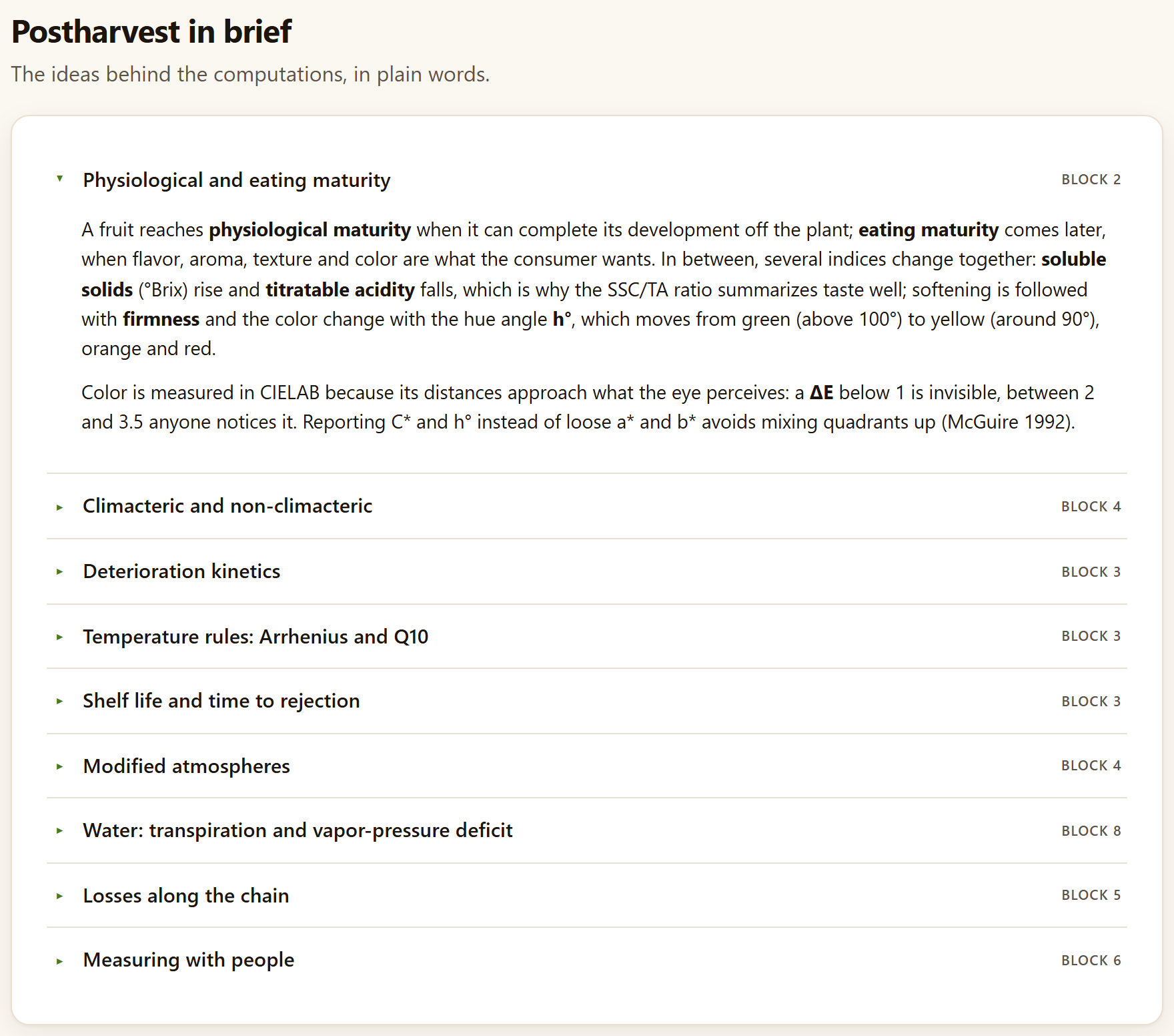
The Postharvest in brief section (The ideas behind the computations, in plain words.) has nine collapsible panels, each with the block where its idea applies. When the home page opens only the first one is expanded; a click on the title opens or closes any of them.
Table 1.5. What each collapsible panel explains
Panel
Block
The idea, in one line
Physiological and eating maturity
2
Soluble solids rise and acidity falls, which is why SSC/TA sums up taste; the hue angle h° moves from green (above 100°) to yellow (around 90°); a ΔE below 1 is not noticed, and between 2 and 3.5 anyone notices it
Climacteric and non-climacteric
4
Climacteric fruit have a peak of respiration and of autocatalytic ethylene and ripen off the plant; respiration releases about 10.7 J per milligram of CO₂
Deterioration kinetics
3
Zero, first or second order; the order is chosen by fitting on the original scale and comparing AIC, not by the R² of a straight line
Temperature rules: Arrhenius and Q10
3
ln k = ln A − Eₐ/(RT); Q10 is not constant; accelerated tests assume that the mechanism does not change with temperature
Shelf life and time to rejection
3
By an attribute limit or by the rejection of each fruit; fruit still sound at the end are censored, not discarded
Modified atmospheres
4
The steady state matches what the produce respires with what permeates the film; β = PCO₂/PO₂ fixes the line of possible atmospheres
Water: transpiration and vapor-pressure deficit
8
The fruit loses water in proportion to the vapor-pressure deficit; 3 to 10% of weight lost is already enough to make it shrivel
Losses along the chain
5
Losses are computed on what enters each stage; in kilograms the first stages weigh most, in money the last ones
Measuring with people
6
Discrimination, affective and descriptive tests; Thurstonian d′ measures the size of a difference; Williams orders avoid order bias
Each chapter of this manual comes back to these ideas in more detail in its “Theory in brief” boxes, next to the tool that uses them.
Figure 1.4.Postharvest in brief, with the first panel expanded. To the right of each title, the block where the idea is used.
1.7What it does not do
Four boxes say plainly what cannot be expected of the program. They are the same limits that Section I.10 of the introduction tabulates, which adds two more (it does not simulate package dynamics or read instruments):
It does not replace measurement.The models summarize data; extrapolating far from the temperatures, times or cultivars measured is the user’s responsibility, and the app warns when it happens. The most visible warning is in Block 3›Temperature, which flags as an extrapolation any storage temperature outside the measured ones.
It brings no trade standards.The tables of sizes, permeabilities and compatibility are indicative and editable: use those of your standard, your film and your cultivar. The size-grade templates in Chapter 2 are an example of this.
It does not model non-isothermal kinetics.Predictions are at constant temperature; variable temperature histories need k(T(t)) integrated over time.
It uploads nothing.There is no server, account or connection: what you save is a project file on your computer.
1.8References and how to cite
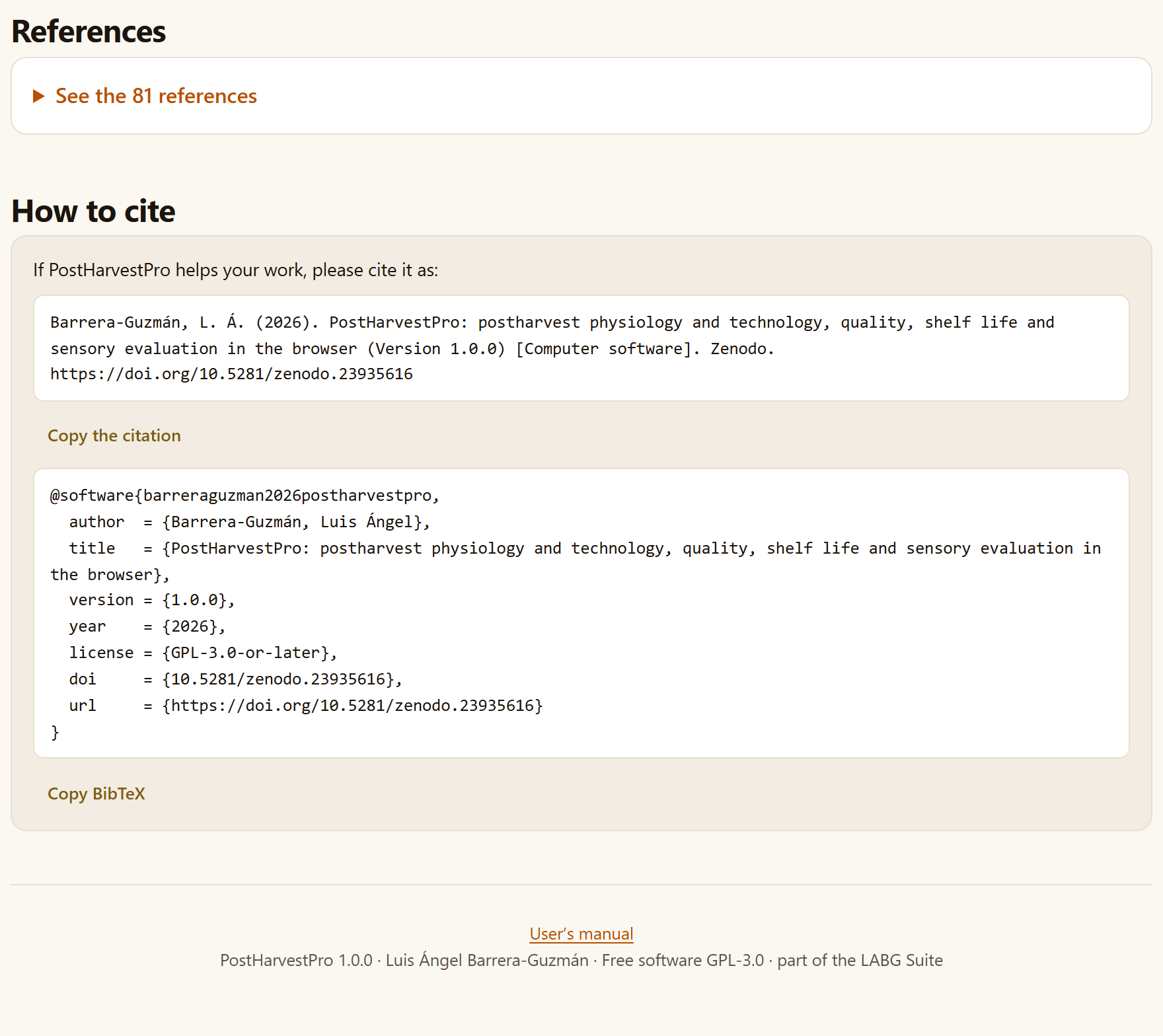
The last two sections of the home page are the bibliography and the citation. In References, the See the 81 references panel opens the complete list of the works cited by the methods, in alphabetical order; it is the same list that Appendix F gathers, there grouped by topic.
How to cite begins with If PostHarvestPro helps your work, please cite it as: and gives the program’s citation in two forms, each with its button:
The reference, in the language of the interface, copied with Copy the citation:
Barrera-Guzmán, L. Á. (2026). PostHarvestPro: postharvest physiology and technology, quality, shelf life and sensory evaluation in the browser (Version 1.0.0) [Computer software]. Zenodo. https://doi.org/10.5281/zenodo.23935616
The BibTeX entry, with the key barreraguzman2026postharvestpro, the English title, version 1.0.0, the year, the license GPL-3.0-or-later, the DOI and the address; it is copied with Copy BibTeX.
When you copy, a brief notice confirms Copied. The citation carries the Zenodo concept digital object identifier (DOI), which always resolves to the latest version. The same citation is at the end of Block 9 (Section 9.7) and at the end of every report. The home page closes with a footnote holding the User’s manual link, which opens this manual in another tab (with the interface in Spanish it reads Manual de usuario (en español) and opens the Spanish edition), and a line saying that PostHarvestPro 1.0.0 is free software (GPL-3.0) and part of the LABG Suite.
Figure 1.5.References and How to cite, at the end of the home page, and the footnote with the link to the manual.
✓Where to start
If it is the first time you open the app
then press Start with an example → and go through Chapter 2 with the mango; then open the same mango in Block 3 (Open in 3 · Kinetics).
If you have measurements of a lot over time
then start in Block 2 to summarize them and go on to Block 3 for their shelf life and to Block 7 to compare the treatments.
If your question is about respiration, losses, tasting or packaging
then go straight to its block (4, 5, 6 or 8): each one works with its own table or with its typed fields.
If you do not know what columns your table should have
then download the ⤓ CSV of the most similar example and use it as a template.
If you are going to publish the results
then cite the program from here or from Block 9, and also cite the method of each result.
They are guides for finding your way, not a mandatory order.
✕When something goes wrong
An Open in … button takes me to the tab, but I see no results. The results are below the data input; scroll down or use the In this block list. The copy buttons do nothing. Some browsers do not allow the clipboard on pages opened as a local file; select the citation text and copy it by hand, or open the app with Open PostHarvestPro.bat (Section I.5). The illustration is not animated. Animations are turned off (sparkles button in the top bar) or your system asks for reduced motion; it does not affect any computation. I lost what I had loaded when I opened an example. The example replaces the tool’s table; if you saved the project, open it again in Block 9.
2
Chapter two · Block 2
Quality and maturity
Measuring is the first step of any postharvest work: how much the fruit has softened, how much sugar and how much acidity it has, what color it is, how much damage it shows and how large it is. Block 2 summarizes those measurements by lot and by time, converts and compares colors in CIELAB, solves the everyday laboratory calculations and turns damage scales and size grades into indices and percentages. Its results are read on their own or passed on to Block 3, which models their rate, and to Block 7, which decides whether the differences are real.
2.1The data input of every tool
2.2Quality summary
2.3Color: converter and indices
2.4Difference between two colors and the color of your data
2.5Acidity, moisture, firmness and weight loss
2.6Ripeness and damage scales
2.7Size grades
The block title sums it up in one line: Quality indices, CIELAB color, laboratory calculators, scales and size grades. Its five tabs are Quality summary, Color, Acidity, moisture and firmness, Ripeness and damage scales and Size grades. Three of them read a table and the other two are filled in by typing; all of them are recomputed as soon as you change a value. The thread of this chapter is the example mango: 72 simulated fruit, four per temperature and day, stored at 13, 20 and 25 °C.
2.1The data input of every tool
All the tools of the app that analyze a table—from the quality summary to the trials of Block 7—receive the data in the same box. It is explained here once; the other chapters only say which roles each tool asks for.
123456789
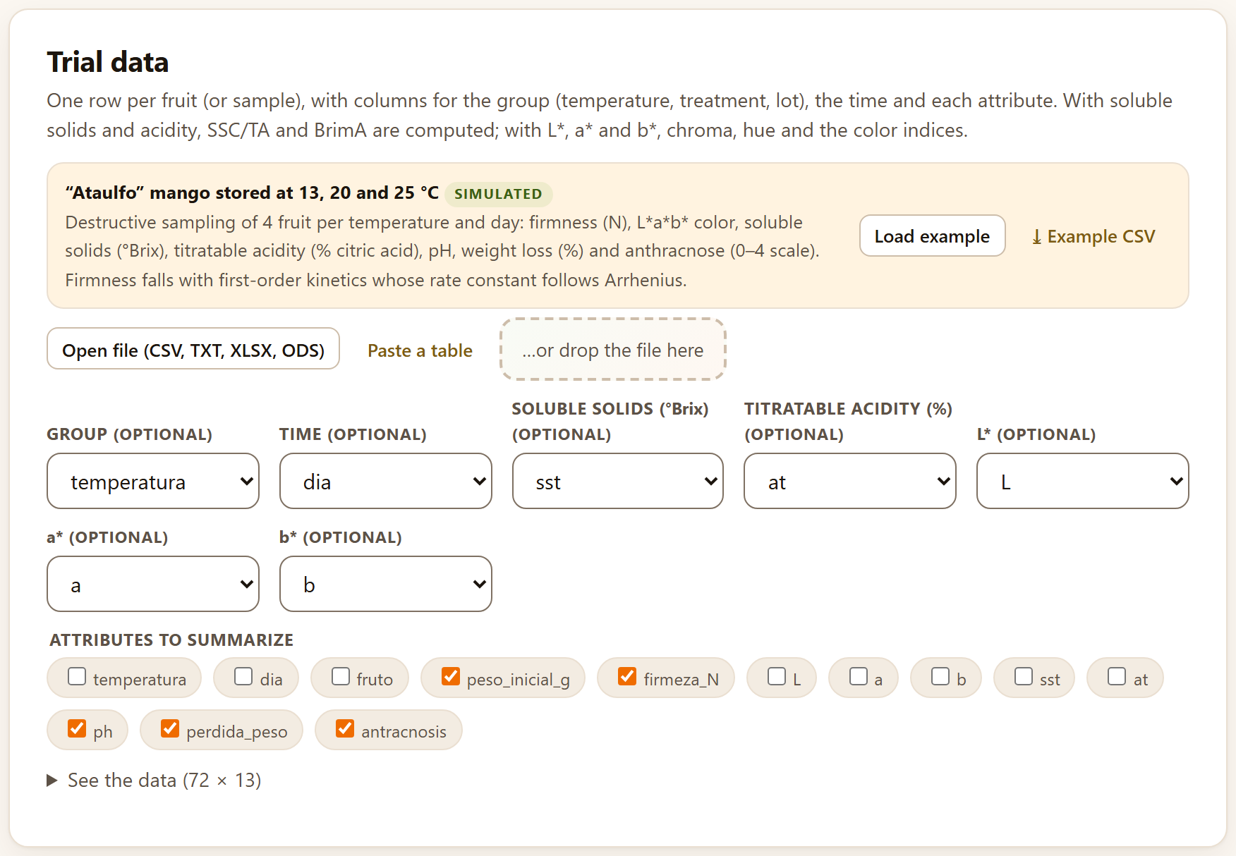
Figure 2.1.Block 2›Quality summary›Trial data with the example mango loaded. The numbers refer to the list below.
1The example strip. The name of the data set, the SIMULATED tag and its description. It is always there, even if you do not load it: it shows the layout of a table the tool understands.
2Load example. Loads the data set and runs the analysis. It is what the Open in … buttons of the home page press for you.
3⤓ Example CSV. Downloads the example table; it serves as a template for yours.
4Open file (CSV, TXT, XLSX, ODS). Reads a file from your computer: CSV, TSV or TXT separated by comma, semicolon or tab, or an XLSX, XLSM or ODS workbook. If the workbook has several sheets, a selector appears on the right to choose which one to read.
5Paste a table. Opens a box where you paste the cells copied from a spreadsheet, with the column names in the first row, and read them with Use the pasted table.
6…or drop the file here. Drag the file from your file explorer and drop it on the dashed box.
7The roles. One list for each piece of data the tool needs, with all the columns of the table. The app proposes the matching one by its name; you confirm it or change it. Roles marked (optional) can be left at — none —.
8A role with several columns. Some tools ask for several columns for the same role, with one check box per column; here, Attributes to summarize.
9See the data (72 × 13). Expands the table that was read, with its number of rows and columns, so that you can check it was read correctly (it shows the first 200 rows).
When a table is loaded, the analysis runs by itself, and runs again every time you change a column. If a required role is missing, the app does not compute and says so below the buttons: Choose the column for: …, with the name of the role. Other messages in the same place are The table has no rows with data. and Could not analyze: …, followed by the cause.
!Always in long format
One row per observed unit—a fruit, a jar, a consumer with a product—and one column per variable. The example mango has one row per fruit with its temperatura, its dia and its attributes; not one column per day. Empty cells, NA or — are taken as missing.
What the results have in common
Below the data, every tool shows its results with the same pieces, which the rest of the manual only names:
Piece
What it is and what you do with it
Tiles
The numbers that matter, in boxes with their label and a line of detail. A tile with a colored border calls attention: amber for a warning or the worst case, green for the best
Reading
A cream box with a green border that says in words what the numbers mean for the product
Figures
Each in its own box with a title. In its corner, Download SVG (arrow), Download PNG at 300 ppi (picture) and, if the figure has one, Figure data (CSV) (grid). When you hover over it, ✎, the figure editor, and the figure studio button also appear; in the studio the same downloads appear with their names: SVG, PNG at 300 ppi and Data (CSV) (Chapter 9, Section 9.5)
Tables
With the ⤓ CSV and ⤓ XLSX buttons below them, to take them to a spreadsheet
Method and source:
The last line: the method that was applied and the works that define it, with author and year (Appendix F gives the full reference)
Every analysis you run also leaves its section in the report of Block 9 (Chapter 9), with its figures, its table and its reading.
2.2Quality summary
The first tab summarizes any set of quality attributes by group and by time: the mean with its dispersion, the course of one variable and the change between the first and the last sampling. It is the table that goes into any trial report, before modeling or comparing.
The Trial data card asks for one row per fruit or per sample. All its roles are optional: Group (temperature, treatment, lot), Time, Soluble solids (°Brix), Titratable acidity (%), L*, a*, b* and Attributes to summarize. With soluble solids and acidity, the app computes SSC/TA and BrimA for each fruit; with L*, a* and b*, chroma, hue, the citrus color index and the browning index (Section 2.3). Those computed variables are added to the attributes you tick.
With the mango, the app proposes temperatura as group, dia as time, sst, at, L, a and b in their roles and, as attributes, the numeric columns left free except those that identify the unit (fruto): peso_inicial_g, firmeza_N, ph, perdida_peso and antracnosis.
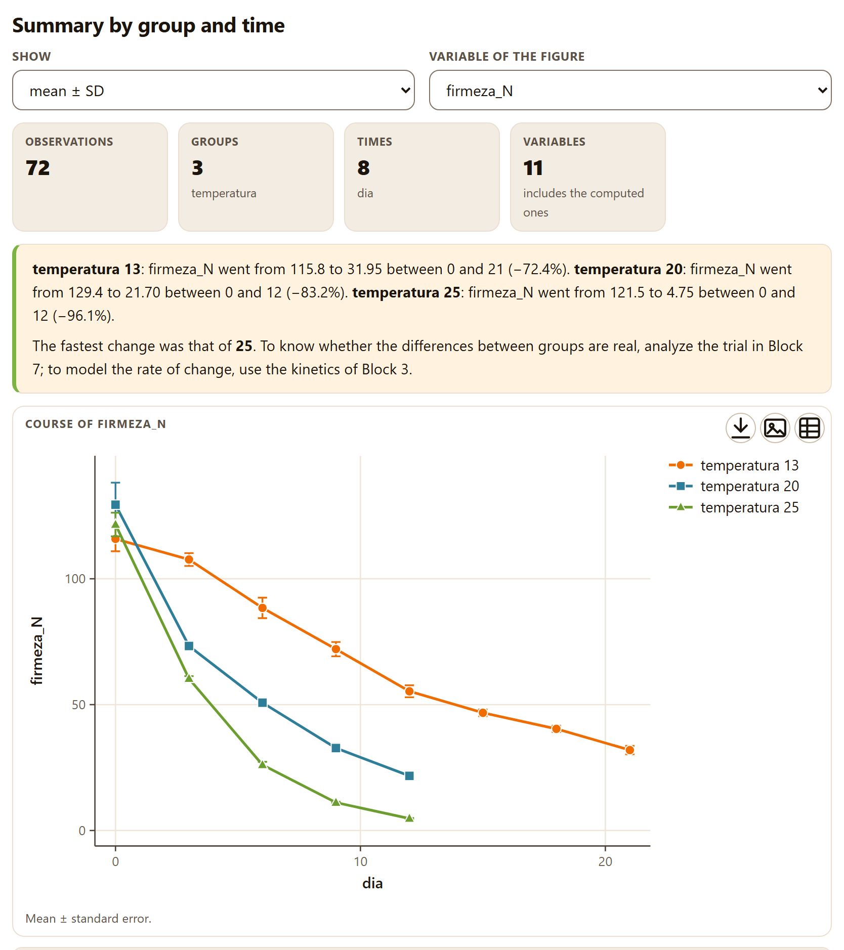
Figure 2.2.Summary by group and time with the example mango. Firmness falls at all three temperatures, faster the warmer it is; at 20 and 25 °C the trial ends on day 12, at 13 °C on day 21. The table, which follows below the figure, is not shown.
Above the results there are two controls. Show chooses what goes with the mean in the table: mean ± SD (the default), mean ± SE or mean and 95% CI, which writes the interval in square brackets. Variable of the figure chooses which variable is drawn; it opens with firmeza_N if there is one.
Tiles.Observations 72; Groups 3 (temperatura); Times 8 (dia: the distinct values of the whole table); Variables 11, with the note includes the computed ones: the five ticked plus SSC/TA, BrimA, chroma, hue and the two color indices.
Reading. The change of the figure variable between the first and the last time of each group, as a value and as a percentage: at 13 °C firmness went from 115.8 to 31.95 N between days 0 and 21 (−72.4%); at 20 °C, from 129.4 to 21.70 N between 0 and 12 (−83.2%); at 25 °C, from 121.5 to 4.75 N between 0 and 12 (−96.1%). It ends by pointing out the group that changed fastest, here 25, and refers to Block 7 to find out whether the differences are real and to Block 3 to model their rate.
Figure.Course of firmeza_N: the mean of each group at each time with standard-error bars (Mean ± standard error.). If you choose no time, the figure is a bar chart, one bar per group.
Table. One row per group and time—18 for the mango: eight times at 13 °C and five at 20 and at 25 °C—with its n and one column per variable. For instance, at 13 °C on day 0: firmness 115.8 ± 9.79 N, SSC/TA 7.39 ± 0.512 and hue 109.2 ± 1.42°; on day 21, SSC/TA 54.12 ± 8.59 and hue 79.77 ± 2.01°.
The Method and source: line reads Titratable acidity by titration (AOAC 942.15) · BrimA: Jordan et al. 2001 · Color: CIE 2018; McGuire 1992 · CCI: Jiménez-Cuesta et al. 1981 · BI: Palou et al. 1999: the last two are the sources of the color indices the summary computes.
θTheory in brief: SSC/TA and BrimA
As it ripens, the fruit accumulates sugars and consumes acids: soluble solids (SSC, in °Brix) rise and titratable acidity (TA, in % of the dominant acid) falls. Their ratio sums up taste, but it exaggerates when acidity is very low. BrimA corrects it by subtracting acidity with more weight, because the tongue perceives it more strongly than sugar (Jordan et al. 2001):
SSC/TA = SSC ∕ TA BrimA = SSC − 2·TA
In the example mango at 13 °C, SSC/TA goes from 7.39 to 54.12 in 21 days: the fruit has become much sweeter to the palate.
2.3Color: converter and indices
The Color tab has three cards. The first, Color converter, translates a color between its three notations and computes the indices used in the postharvest literature.
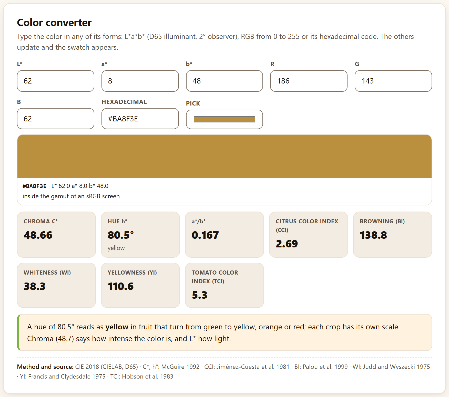
Its hint says: Type the color in any of its forms: L*a*b* (D65 illuminant, 2° observer), RGB from 0 to 255 or its hexadecimal code. The others update and the swatch appears. The fields are L*, a*, b*, R, G, B, Hexadecimal and Pick, which opens the system color picker. It opens with L* 62, a* 8 and b* 48, the yellow of a ripe mango.
Figure 2.3. The Color converter with its starting values: the color is #BA8F3E (R 186, G 143, B 62), inside the gamut of an sRGB screen.
Below the fields, the swatch of the color with its code and its coordinates, and a note: inside the gamut of an sRGB screen or, if the color cannot be displayed, outside the sRGB gamut: shown is the nearest with the same L* and h°. The eight tiles with the starting values are:
Table 2.1. The converter indices for L* 62, a* 8, b* 48
Tile
Value
Formula and source
Chroma C*
48.66
C* = √(a*² + b*²): the intensity of the color (McGuire 1992)
Hue h°
80.5°
h° = atan2(b*, a*), from 0 to 360°; with its reading, yellow
a*/b*
0.167
From negative (green) to positive (red); widely used in tomato and mango
Citrus color index (CCI)
2.69
CCI = 1000·a* ∕ (L*·b*): negative green, near 0 at color break, positive orange (Jiménez-Cuesta et al. 1981)
Browning (BI)
138.8
BI = 100(x − 0.31) ∕ 0.17, with x = (a* + 1.75L*) ∕ (5.645L* + a* − 3.012b*) (Palou et al. 1999)
Whiteness (WI)
38.3
WI = 100 − √((100 − L*)² + a*² + b*²), the form used for fresh-cut products (Judd and Wyszecki 1975)
Yellowness (YI)
110.6
YI = 142.86·b* ∕ L* (Francis and Clydesdale 1975)
Tomato color index (TCI)
5.3
TCI = 2000·a* ∕ (L*·C*) (Hobson et al. 1983)
The reading puts the hue into words: A hue of 80.5° reads as yellow in fruit that turn from green to yellow, orange or red; each crop has its own scale. The words come from fixed cuts of the angle: green from 105°, green-yellow from 85 to 105°, yellow from 70 to 85°, orange from 50 to 70°, red-orange from 25 to 50° and red below. They are a general guide, not the scale of your crop. The reading adds the chroma (Chroma (48.7) says how intense the color is, and L* how light.), and the method line gives the source of each tile: CIE 2018 (CIELAB, D65) · C*, h°: McGuire 1992 · CCI: Jiménez-Cuesta et al. 1981 · BI: Palou et al. 1999 · WI: Judd and Wyszecki 1975 · YI: Francis and Clydesdale 1975 · TCI: Hobson et al. 1983.
iWhy C* and h° and not a* and b* on their own
The same change in a* means different things depending on the sign of b*, and averaging angles or ratios of colors from different quadrants misleads. Chroma and hue separate what the eye distinguishes—how intense and what color—and can be compared between fruit (McGuire 1992). The converter works with the D65 illuminant and the 2° observer; if your colorimeter uses another illuminant, its L*a*b* are not directly comparable.
2.4Difference between two colors and the color of your data
Difference between two colors
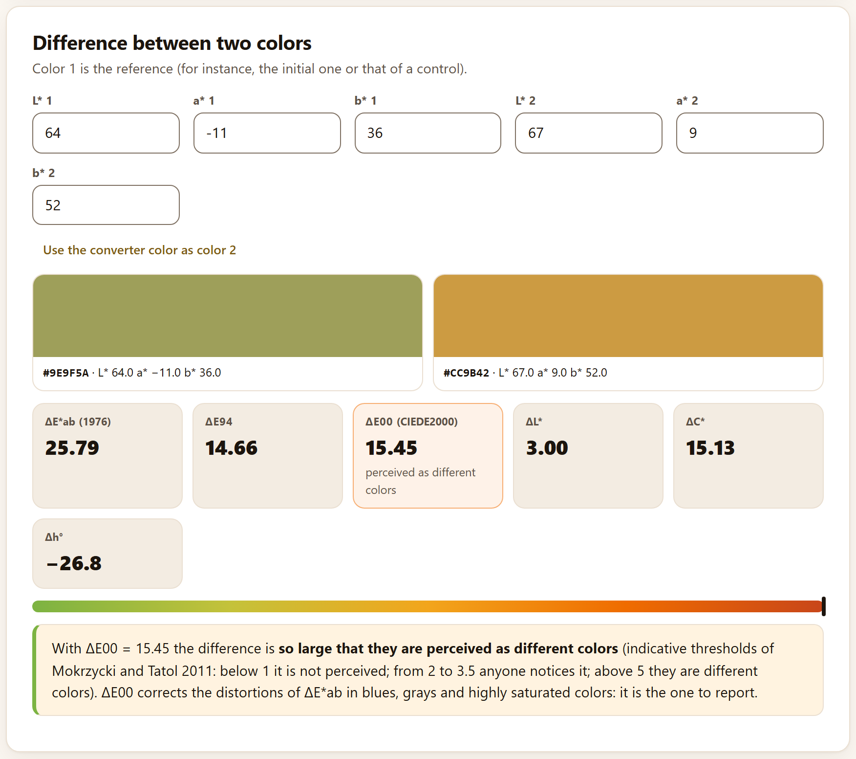
The second card measures how distinguishable two colors are. Its hint says Color 1 is the reference (for instance, the initial one or that of a control). The fields are L* 1, a* 1, b* 1, L* 2, a* 2 and b* 2; they open with the green of a freshly harvested mango (64, −11, 36) and a ripe yellow (67, 9, 52). The Use the converter color as color 2 button copies the color from the previous card.
Figure 2.4.Difference between two colors with the starting values. The bar at the bottom runs from green (no difference) to red; its marker is at the end because ΔE00 exceeds 8.
The tiles give the three difference formulas and their components: ΔE*ab (1976) 25.79, ΔE94 14.66 and ΔE00 (CIEDE2000) 15.45, the latter with its reading (perceived as different colors) and highlighted when it reaches 3.5; and ΔL* 3.00, ΔC* 15.13 and Δh° −26.8°, the difference in hue angle (color 2 is 26.8° less green). The reading puts it in one sentence—With ΔE00 = 15.45 the difference is so large that they are perceived as different colors—, gives the guide thresholds and recommends reporting ΔE00. In that sentence, the two highest grades read clear and so large that they are perceived as different colors; in the tile, as in the table below.
✓Decision rule: is the color difference noticed?
ΔE00
What the app says
below 1
not perceptible
from 1 to 2
perceptible only to a trained observer
from 2 to 3.5
perceptible to any observer
from 3.5 to 5
clear difference
5 or more
perceived as different colors
Guide thresholds of Mokrzycki and Tatol (2011). ΔE00 corrects the distortions of ΔE*ab in blues, grays and highly saturated colors: in the example, ΔE*ab overstates the difference by more than 10 units.
The color of your data
The third card reads a table with L*, a* and b* per fruit: L*, a* and b* columns, with group and time: the mean color of each group at each time, its ΔE00 from the group’s initial color and the course of hue. It asks for L*, a* and b* (required) and Group and Time (optional). Its Load example loads the mango.
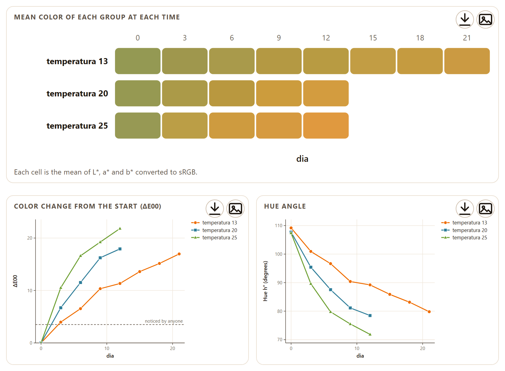
Figure 2.5.The color of your data with the example mango: the strip of mean colors (top), the color change from day 0, with the 3.5 line noticed by anyone (left), and the hue angle (right).
The app averages L*, a* and b* of the fruit of each group and time, converts that mean into a screen color and computes its chroma, its hue and its ΔE00 with respect to the first time of the same group. The three figures are Mean color of each group at each time (Each cell is the mean of L*, a* and b* converted to sRGB.), Color change from the start (ΔE00) and Hue angle; below them comes the table with L*, a*, b*, C*, h°, ΔE00 and a Swatch of the color with its code.
▸Worked example: the mango changes color
At 13 °C the mean hue of the mango falls from 109.2° on day 0 to 79.8° on day 21—from green to yellow—and its ΔE00 reaches 16.96. At 25 °C the change is faster and larger: the hue reaches 71.9° and ΔE00 21.81 on day 12. At all three temperatures the difference from the initial color is already perceptible to anyone (ΔE00 > 3.5) from day 3: 3.96 at 13 °C, 6.70 at 20 °C and 10.52 at 25 °C.
The method line cites CIE 2018 (CIELAB, D65) · ΔE00: Sharma et al. 2005 · C*, h°: McGuire 1992.
2.5Acidity, moisture, firmness and weight loss
The Acidity, moisture and firmness tab brings together four laboratory calculators that read no tables: you type the readings and the result appears at once. They open with example values typed in.
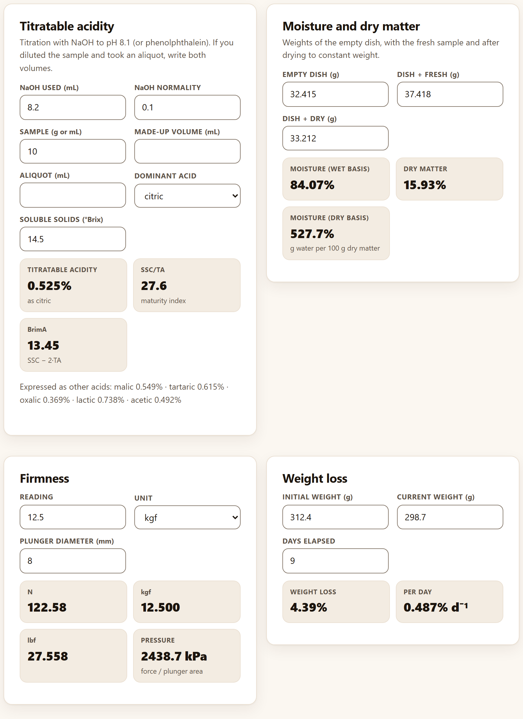
Figure 2.6. The four calculators with their starting values.
Titratable acidity
For a titration with NaOH to pH 8.1 or to the phenolphthalein end point. The fields are NaOH used (mL) 8.2, NaOH normality 0.1, Sample (g or mL) 10, Made-up volume (mL) and Aliquot (mL)—empty: only if you diluted the sample and took part of it—, Dominant acid (citric, malic, tartaric, oxalic, lactic or acetic) and Soluble solids (°Brix) 14.5.
TA (%) = VNaOH · N · meq · (made-up volume ∕ aliquot) · 100 ∕ sample
The milliequivalent is that of the chosen acid: 0.064 for citric (citrus, mango, papaya, tomato, strawberry, pineapple), 0.067 for malic (apple, pear, peach, plum, banana), 0.075 for tartaric (grape, tamarind), 0.045 for oxalic, 0.090 for lactic and 0.060 for acetic. With the starting values, acidity is 0.525%as citric, SSC/TA 27.6 (maturity index) and BrimA 13.45. Below, the same acidity Expressed as other acids: malic 0.549%, tartaric 0.615%, oxalic 0.369%, lactic 0.738% and acetic 0.492%.
Moisture and dry matter
With the three weighings of the dish (Weights of the empty dish, with the fresh sample and after drying to constant weight.): Empty dish (g) 32.415, Dish + fresh (g) 37.418 and Dish + dry (g) 33.212. They give Moisture (wet basis) 84.07%, Dry matter 15.93% and Moisture (dry basis) 527.7%, that is, grams of water per 100 g of dry matter.
Firmness
Converts a penetrometer reading: Reading 12.5, Unit (N, kgf, lbf or gf; it opens at kgf) and Plunger diameter (mm) 8. It gives the force in N (122.58), kgf (12.500) and lbf (27.558), and the Pressure on the plunger area, 2438.7 kPa. Pressure lets you compare readings taken with different plungers; force does not.
Weight loss
Initial weight (g) 312.4, Current weight (g) 298.7 and Days elapsed 9 give a Weight loss of 4.39%, computed on the initial weight, and 0.487% per day. When the loss reaches 5%, the tile turns amber and warns that it is near the limit at which many fruit shrivel.
iThe calculators leave no section in the report
They are one-off laboratory calculations: their results do not pass on to Block 9. If you want the weight loss or the acidity of a whole trial in the report, put them as columns of your table and analyze them in Quality summary or in Block 7.
2.6Ripeness and damage scales
Many attributes are rated by eye on a scale of classes: the ripeness stage from the skin color, the severity of a spot, the progress of a rot. The Ripeness and damage scales tab turns those ratings into a weighted index, the incidence and the percentage of marketable fruit of each lot.
The The scale card has an editable table with the Value and the Description of each class (Each class with its value (0 = sound, or the first grade) and its description. Edit it or pick a template.). It opens with the Damage 0–4 template—Sound, Slight (< 5% of the surface), Moderate (5–15%), Severe (15–30%) and Very severe (> 30%)—; the other two are Ripeness 1–5 (from Mature green to Overripe) and Decay 0–3 (from No decay to Rotten fruit). + Add row and × add or remove classes. Below, Market tolerance (highest class accepted) chooses the highest class that still sells; it opens at the second class, here class 1.
The The data card accepts two inputs. The first is a table with Class of each fruit (required) and Group and Time (optional); each combination of group and time is a lot. The second, in the …or type counts by lot panel, are counts typed by hand, one lot per line—for instance Lot A: 50, 20, 15, 10, 5—, which are read with Use the counts. If any rating matches no class of the scale, a warning says how many were left out of the count.
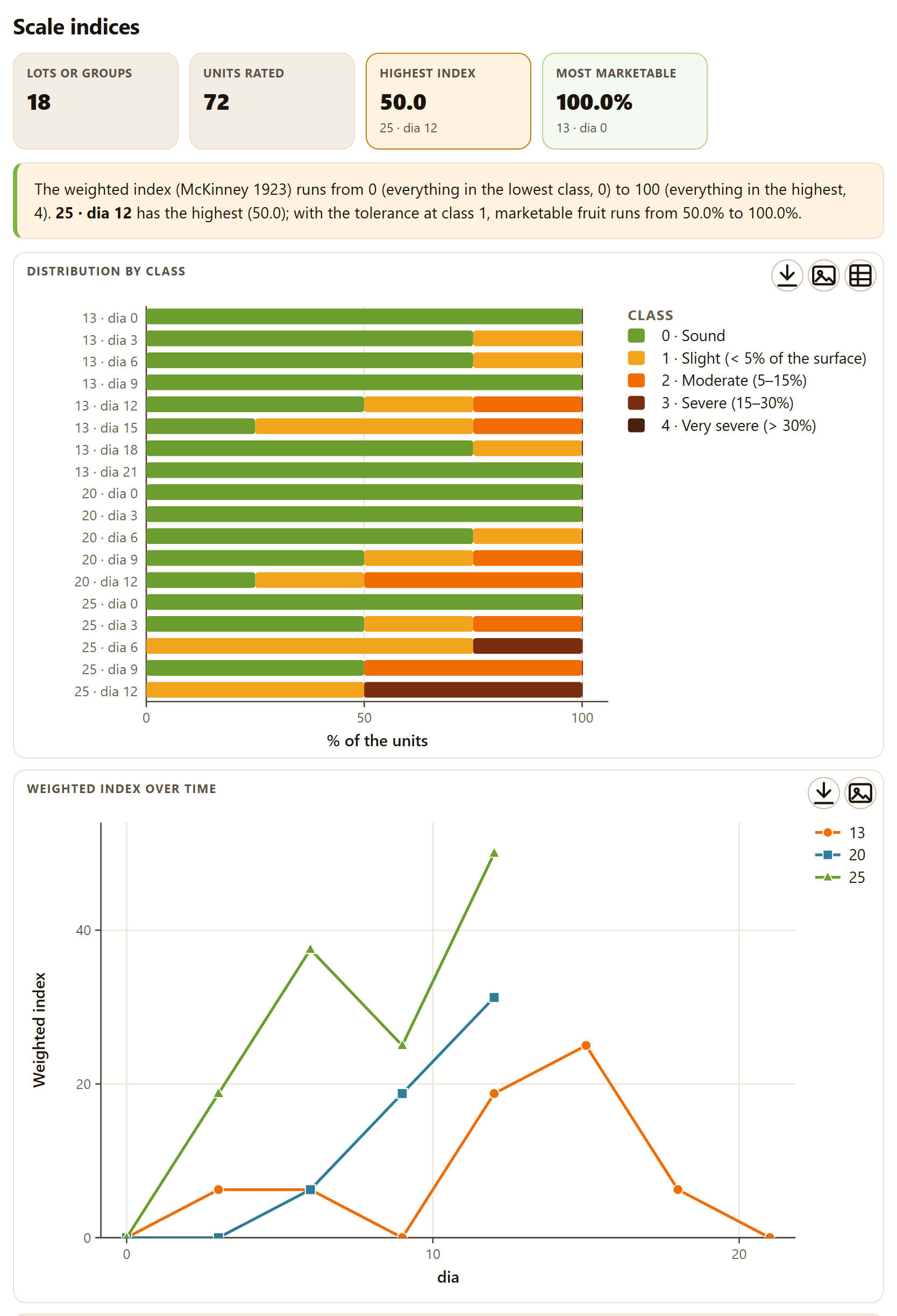
Figure 2.7.Scale indices with the anthracnose of the example mango (scale Damage 0–4, tolerance at class 1). Each lot is one temperature on one day. The table, below the figures, is not shown.
With the mango, the app takes antracnosis as the class, temperatura as group and dia as time: 18 lots of four fruit. The tiles read Lots or groups 18, Units rated 72, Highest index 50.0 (25 · dia 12, in amber) and Most marketable 100.0% (the first lot to reach it, 13 · dia 0, in green). The reading starts with the range of the index for the chosen scale—The weighted index (McKinney 1923) runs from 0 (everything in the lowest class, 0) to 100 (everything in the highest, 4).—and adds that, with the tolerance at class 1, marketable fruit runs from 50.0% to 100.0%. The figures are Distribution by class, one stacked bar per lot, and, when there are group and time, Weighted index over time, one line per group. The table gives for each lot its N, the percentage in each class, the Index, the Mean grade, the Incidence and the Marketable percentage.
θTheory in brief: the McKinney index
The weighted index weights each fruit by its class and expresses it as a percentage of the maximum possible damage (McKinney 1923):
Index = 100 · Σ(class · n) ∕ (N · maximum class)
The mean grade is Σ(class · n) ∕ N; the incidence, the percentage of units above the lowest class; and the marketable fruit, the percentage at the tolerance class or below. In the 25 °C lot on day 12, two fruit in class 1 and two in class 3 give 100 · (2·1 + 2·3) ∕ (4 · 4) = 50.0, an incidence of 100% and 50% marketable.
!With scales that start at 1
The formula divides by the maximum class, so the index only falls to 0 on scales that start at 0, like those for damage and decay. With Ripeness 1–5, a whole lot in class 1 gives 20, and the reading says so: runs from 20 (everything in the lowest class, 1) to 100 (everything in the highest, 5). Compare indices only between lots rated with the same scale.
The method line is Weighted index: McKinney 1923. The analysis is redone with the same data—the table or the typed counts—as soon as you choose another template, edit a class or change the tolerance.
!The scale must match your ratings
If you apply Ripeness 1–5 to the anthracnose of the mango, rated from 0 to 4, two warnings appear: 46 grades match no class of the scale and are not counted. and 6 lots have no grade within the classes of the scale and are left out: 13 · dia 0, 13 · dia 9, 13 · dia 21, 20 · dia 0, 20 · dia 3, 25 · dia 0. The result is left with 12 lots and 26 units, the highest index is 40.0 (25 · dia 9) and marketable fruit runs from 0.0% to 100.0%. Choose or type the scale you rated with. Two other warnings in the same place: The class column has no number at all. and, if you delete every class, The scale needs at least one class with its value.
2.7Size grades
The last tab sorts the fruit by size: how many fall in each grade, which one is the most frequent and how many are left outside the classes.
The The classes card has an editable table with Grade, Minimum and Maximum: Each grade with its minimum (included) and maximum (excluded, except in the last class), in the unit of your data. The templates are indicative: use those of your standard. There are three templates:
Table 2.2. The size-grade templates
Template
Classes
By weight (g)
Small 0–200, Medium 200–280, Large 280–360 and Extra large 360–600 g (the starting one)
Fruit per 4 kg box
Count 8 to Count 20: count k corresponds to fruit of about 4000 ∕ k g, and the limits are the midpoints between neighboring counts (Count 14: 268–310 g)
By diameter (mm)
< 57 mm, 57–67 mm, 67–77 mm, 77–87 mm and > 87 mm
The The fruit card asks for Weight or diameter of each fruit and, optionally, a Group (lot, variety, origin). With the mango, the app takes peso_inicial_g.
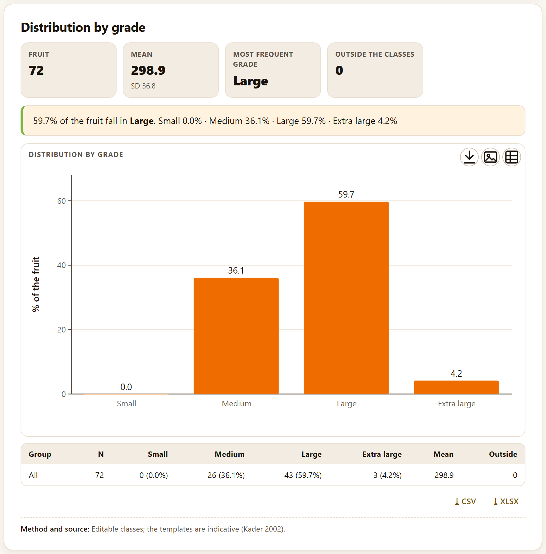
Figure 2.8.Distribution by grade of the initial weight of the 72 mangoes of the example, with the By weight (g) template.
The tiles read Fruit 72, Mean 298.9 g (SD 36.8), Most frequent gradeLarge and Outside the classes 0. The reading distributes the fruit: Large 59.7%, Medium 36.1%, Extra large 4.2% and Small 0.0%. With the Fruit per 4 kg box template, the most frequent grade is Count 14 (44.4%), followed by Count 12 (36.1%). If you choose a group, the figure shows one series of bars per group and the table one row per group. The method line recalls that the classes are editable and the templates a guide only (Kader 2002).
!The classes must be in the unit of your data
If you sort weights with the By diameter (mm) template, all 72 mangoes fall outside the classes: the Outside the classes tile reads 72 and asks you to check the limits, the most-frequent-grade tile is left at —, there is no figure and, instead of the reading, a warning explains the mismatch: No fruit falls inside the classes: the data run from 230 to 369 and the classes from 0 to 150. Check the limits and the unit (weight or diameter). If only some fruit fall outside, the reading ends with their percentage (· outside the classes …).
✓Decision rule: which Block 2 tool to use
If you have attributes measured in several lots and times
thenQuality summary; afterward, Block 3 for their rate and Block 7 to compare.
If you have L*a*b* readings per fruit
thenThe color of your data, and report C*, h° and ΔE00, not a* and b* on their own.
If ΔE00 between two treatments is less than 2
then the consumer will hardly notice the color difference, even if it is statistically significant.
If you rated by eye with classes
thenRipeness and damage scales, with the tolerance of your market.
If weight loss exceeds 5%
then check the humidity of the store and the package (Block 8).
The thresholds are a guide only; the standard of your product and your market prevails.
✕When something goes wrong
The summary has one row per fruit instead of per time. The time column is at — none — or the group points to the fruit column; check the roles. Identification columns appear among the variables. Untick their box in Attributes to summarize. The colors look odd. Check that L*, a* and b* are not swapped (L* runs from 0 to 100) and that your colorimeter uses D65 and 2°. Acidity comes out ten times larger. You diluted the sample and did not type the made-up volume and the aliquot, or the other way around. Lots are missing from the scale indices. Their ratings do not match the class values (for instance, 1.5 on an integer scale, or a 1-to-5 scale with ratings from 0 to 4); the warnings in The data say how many ratings were discarded and which lots were left out. All the fruit fall outside the size grades. The classes are in another unit or overlap; the warning gives the range of your data and that of the classes: correct the minimums and maximums.
3
Chapter three · Block 3
Kinetics and shelf life
Knowing that a lot softens is not enough: you need to know how fast, how many days it takes to reach the limit the market accepts, and how much that rate changes with temperature. This block fits the kinetics of deterioration, takes it to Arrhenius to predict shelf life at the storage temperature, extrapolates an accelerated test and, when what you record is the day each fruit is rejected, estimates the time to rejection while counting the fruit that were still sound at the end.
3.1Kinetic models: the three orders
3.2Fit and life to the limit
3.3Temperature: Arrhenius, Q10 and square root
3.4Shelf life at any temperature
3.5Accelerated test
3.6Time to rejection: Kaplan–Meier
3.7Parametric models and time ratios
The block is called Kinetics and shelf life (in the bar, Shelf life) and introduces itself as “Reaction orders, temperature, accelerated tests and time to rejection.” It has four tabs: Kinetic models, Temperature, Accelerated test and Time to rejection. As everywhere in the program, there is no compute button: as soon as there are data, every change to a control redoes the calculations that depend on it.
The four tabs form a path. In Kinetic models you fit an attribute (firmness, color, vitamin C) against time at each temperature; the button Take the k values to the temperature analysis → passes the constants to Temperature, which fits them to Arrhenius and predicts the life at any temperature. Accelerated test does the same when what you have are not constants but shelf lives observed at high temperatures. Time to rejection is a different approach: it does not model an attribute, but the day on which each fruit stops being acceptable. The chapter uses two simulated examples: the example mango (the firmness of 72 fruit at 13, 20 and 25 °C) and the example chayote with two coatings (the days to rejection of 90 fruit).
3.1Kinetic models: the three orders
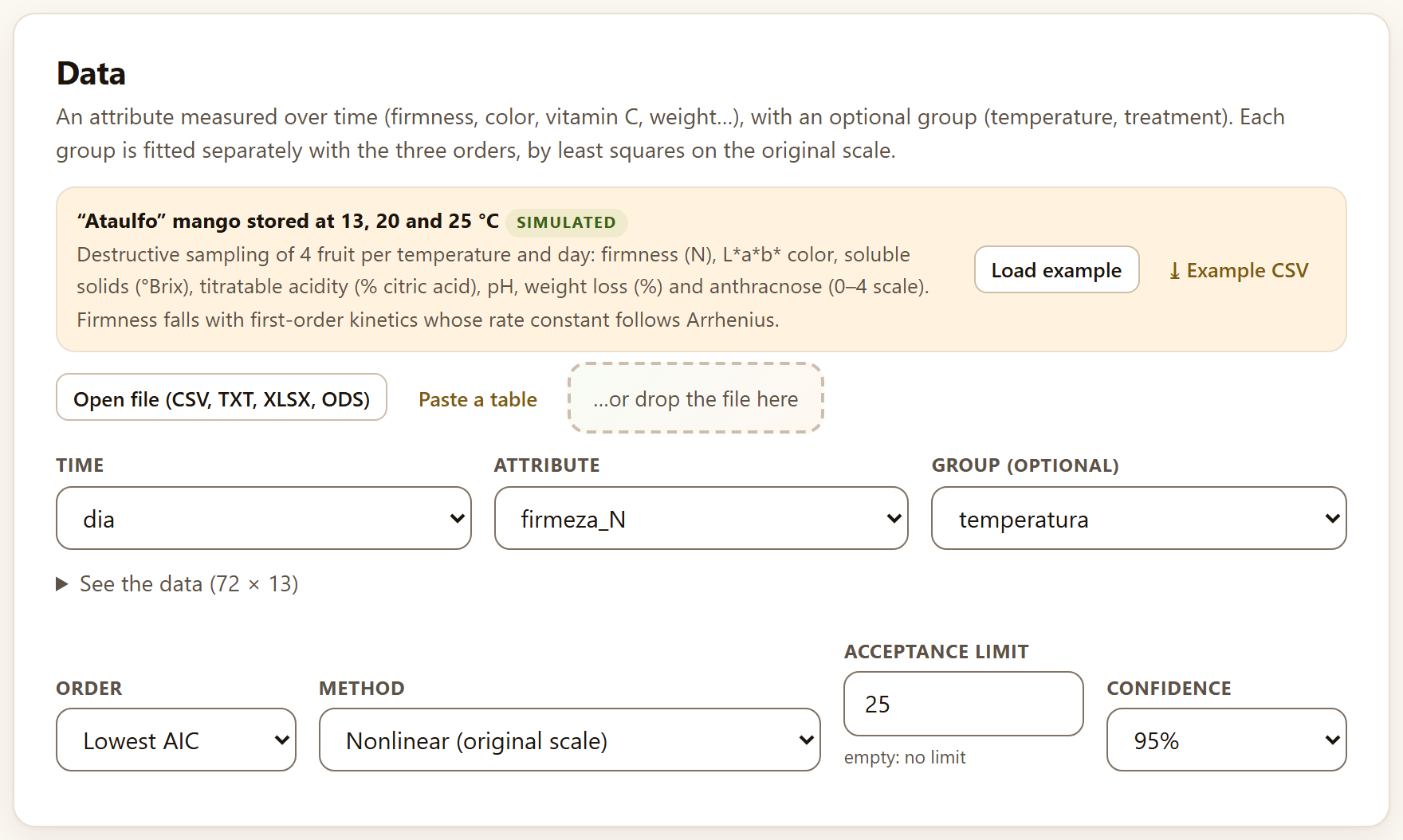
The Data card asks for an attribute measured over time and, if you wish, a group. Its text sums it up: “Each group is fitted separately with the three orders, by least squares on the original scale.”
The column roles are Time (in days, hours or weeks: the app does not convert units, and shelf life comes out in the unit you use), Attribute and Group (optional), which can be the temperature or the treatment. With the example mango (Load example in the strip, or Home›Example data) the app picks dia, firmeza_N and temperatura by itself. The table has thirteen columns (See the data (72 × 13)): you can swap the attribute for color (L, a, b), soluble solids (sst) or weight loss without loading anything again.
Below are four controls:
Table 3.1. The controls of Kinetic models
Control
Default
What it decides
Order
Lowest AIC
Which order is reported in each group; you can also set Zero order, First order or Second order for all of them
Method
Nonlinear (original scale)
How C₀ and k are estimated. Linearized fits the classic straight line (C, ln C or 1/C against t) and is recommended only to compare with older work
Acceptance limit
25 (empty: no limit)
The value of the attribute beyond which the product is no longer acceptable; the time to the limit is computed from it
Confidence
95%
The level of every interval (90, 95 or 99%)
Figure 3.1. The Data card with the example mango: time is dia, the attribute firmeza_N and the group temperatura. Below, the four controls with their default values; the limit of 25 N is the one the app comes with.
The three reaction orders
Almost all quality deterioration is described by one of three forms, which differ in how the rate depends on the value that remains. The app fits all three in each group:
Table 3.2. The three orders, their half-life and their time to the limit L
Order
Model
Half-life
Time to the limit
When it appears
Zero order
C = C₀ − k·t
C₀ / (2k)
(C₀ − L) / k
Changes at a constant rate: nonenzymatic browning, some water losses
First order
C = C₀·e^(−k·t)
ln 2 / k
ln(C₀/L) / k
The rate is proportional to what remains: firmness, vitamins, chlorophyll
Second order
1/C = 1/C₀ + k·t
1 / (C₀·k)
(1/L − 1/C₀) / k
Very fast drops at first that then slow down
A positive k means the attribute goes down; a negative one, that it goes up (the formation of a pigment, for example), and the reading warns about it with “Negative k: the attribute increases with time (formation).”
θTheory in brief · why the original scale and why AIC
The habit of comparing orders by the R² of linearized lines (C, ln C and 1/C against time) has a flaw: each transformation changes the scale of the error, so the three R² are not measured with the same yardstick, and the logarithm or the reciprocal give enormous weight to the small values at the end of the trial. The app fits the three models by nonlinear least squares on the attribute as it was measured (Bates and Watts 1988), so all three share the same residuals and can be compared with the Akaike information criterion (AIC; Burnham and Anderson 2002). AIC rewards a good fit and penalizes parameters; here the three models have two parameters (C₀ and k), so the one with the smallest residual sum of squares wins. The difference from the best, ΔAIC, is turned into the Akaike weight, the relative probability that this order is the best of the three.
The table The three orders (Figure 3.2, bottom) shows for each group and each order its equation, k, the residual sum of squares (RSS), the AIC, the ΔAIC, the Akaike weight and, only as a classic reference, the Linearized R²; the row of the chosen order is shaded green. With the mango, first order wins at all three temperatures: at 13 °C with a weight of 0.971 (ΔAIC 7.02 over zero order), at 20 °C with 0.762 (second order is 2.33 behind and keeps a weight of 0.238) and at 25 °C with 1.000.
Figure 3.2. Top, the chosen fit at each temperature, with C₀ and k (± their standard error), the interval of k, the half-life, the R², the number of fruit and the time to the limit with its interval. Bottom, the comparison of the three orders: first order (in green) has the lowest AIC at all three temperatures. At the foot, the button that takes the k values to the Temperature tab and the methods line.
iNote · linearized R² values are misleading
Look at the Linearized R² column at 13 °C: 0.9455 for zero order and 0.9686 for first order. The difference looks small, but AIC gives first order a weight of 0.971. And at 20 °C the linearized second order has an R² (0.9361) larger than that of zero order (0.8709), although neither comes close to first order. If you choose Linearized in Method, the Mean R² tile flags it with on the linearized scale and the lives change: 25.1, 10.9 and 6.0 days instead of 25.9, 10.4 and 6.3.
3.2Fit and life to the limit
The results card is called Fit and shelf life. Its tiles say how many groups were fitted, which order was chosen and how (by AIC or set by you), the Mean R² and, if there is a limit, the Life to the limit of each group.
With the example mango: 3 groups of temperatura, First order by AIC, mean R² 0.969 and life to the limit 25.9 · 10.4 · 6.3 days (limit 25). The reading in words gives, for each group, the order, k with its interval, the half-life and the day on which the attribute reaches the limit, also with its interval:
Table 3.3. Firmness of the example mango, first order, limit 25 N
Temperature
C₀ (N)
k (d⁻¹)
95% CI of k
Half-life (d)
Days to 25 N
95% CI
13 °C
121.9
0.06119
[0.0557, 0.0666]
11.3
25.9
[24.0, 27.8]
20 °C
127.0
0.1569
[0.137, 0.176]
4.4
10.4
[9.2, 11.5]
25 °C
122.3
0.2508
[0.232, 0.270]
2.8
6.3
[5.9, 6.8]
The intervals of k are written with three significant figures of their larger bound (which is why the one at 13 °C has four decimals and those at 20 and 25 °C, three), and the half-life and the time to the limit with one decimal, the same in the reading and in the table.
The reading closes with two checks: whether AIC chose the same order in every group (“AIC picks the same order in every group.”) and how many times the fastest constant is the slowest (here, 4.1). If the groups do not agree on the order, the reading recommends setting a single one: the k values of different orders do not have the same units and cannot be compared or taken to Arrhenius.
Figure 3.3.Fit and shelf life with the example mango. In the figure, the points are the fruit and the lines the first-order model at each temperature with the confidence band of the mean; the dashed line is the 25 N limit, labeled limit at its left end so as not to hide the curves. The 25 °C curve crosses it around day 6, the 20 °C curve around day 10, and the 13 °C curve, which is still above it when the measurements end (day 21), would cross it around day 26.
How the intervals are computed
The intervals of C₀ and k are Wald intervals with Student’s t and the degrees of freedom of the fit (n − 2), as the reading says: “The intervals are Wald intervals with Student’s t (95%).” The interval of the time to the limit is obtained by the delta method: the time is a function of C₀ and k (Table 3.2), and its variance combines those of the two parameters and their covariance.
The time at 13 °C (25.9 days) falls after the last day measured (21): it is a short extrapolation within the same model. If the attribute never reaches the limit with the chosen model—a zero order with negative k and a lower limit, for example—the reading says does not reach the limit and the tile shows a dash.
Below the reading appear, in smaller type and preceded by the group, the notes of the fit when there are any: for example, “Second order: could not be fitted and is left out of the comparison.” if one of the orders does not converge in that group. With the example mango the three orders are fitted at all three temperatures and no note appears.
Below the figure, the fit table (Figure 3.2, top) repeats these numbers with C₀ and k ± their standard error, the R² on the original scale and the number of fruit in each group (32 at 13 °C, because there it was measured up to day 21; 20 at 20 and 25 °C). Both tables are downloaded with ⤓ CSV and ⤓ XLSX, and the figure with the buttons of its frame (Chapter 2, Section 2.1). The methods are those of Labuza (1984) and van Boekel (2008), with the nonlinear least squares of Bates and Watts (1988) and the AIC of Burnham and Anderson (2002).
▸Worked example · what if I set zero order?
With Order on Zero order, the tile says set by you, the mean R² drops to 0.892 and the lives to the limit become 21.1, 10.3 and 8.1 days. At 13 °C the straight line underestimates the life by almost five days, because it does not curve as firmness drops; at 25 °C it overestimates it by almost two. AIC (Table 3.2) already said that zero order was worse at all three temperatures: setting an order is useful to compare with a published study, not to improve the prediction.
3.3Temperature: Arrhenius, Q10 and square root
The Temperature tab fits the dependence of k on temperature with three models and, with it, predicts shelf life at any temperature. Its input card, “Rate constants at several temperatures,” is an editable table: “Type k (with its standard error, if you have it, to weight) or bring them from the kinetic models.”
The table has the columns Temperature (°C), k and SE of k (optional); + Add row adds one and the × of each row removes it. At least two different temperatures with positive k are needed (three for the square root). Below, the checkbox Weight by the standard error of k (unchecked) and the Reference temperature (°C) (20), at which k is reported.
The tab already opens with the constants of the example mango, fitted as Kinetic models fits them with its default values (order by AIC, nonlinear, 95%): 0.06119 ± 0.0027 at 13 °C, 0.1569 ± 0.0093 at 20 °C and 0.2508 ± 0.0089 at 25 °C, with first order and C₀ = 123.736 (the mean of the three C₀) in the shelf-life section. So opening it directly or reaching it with the button gives the same Eₐ.
The button Take the k values to the temperature analysis →, at the foot of Fit and shelf life, does the same with your data: it first sets the chosen order, the mean of the C₀ and the limit in the shelf-life section, then copies the k and the standard error of each group to the table and opens the tab, so that everything, shelf life included, is computed with the new values. It only works if the group is the temperature written as a number; otherwise it warns “For Arrhenius the group must be the temperature (numbers).” The table shows k with four significant figures and its standard error with two, like the fit table, but it stores and uses the full value until you type another one in the cell.
The three models
θTheory in brief · Arrhenius, Q10 and square root
Arrhenius (1889) assumes that ln k falls in a straight line against the inverse of absolute temperature, with a slope that gives the activation energy Eₐ: the larger Eₐ, the more deterioration speeds up as temperature rises. The app fits the line by least squares on ln k, weighted by (k/SE)² if you tick the box. Q10 is the factor by which k is multiplied with 10 °C more; it is computed between pairs of measured temperatures and, from Eₐ, at any temperature (Taoukis and Labuza 1989): with the same Eₐ, Q10 is larger in the cold than in the heat. The square-root model of Ratkowsky et al. (1982) assumes that √k grows linearly with temperature and crosses zero at a minimum biological temperature, Tmin, below which the process would stop.
With the mango k values, the card Arrhenius, Q10 and square root gives:
Table 3.4. The tiles of Temperature with the k values of the example mango
Tile
Value
What it is
Activation energy
84.2 kJ/mol
With its interval, [−5.5, 173.8]
k (20.0 °C)
0.1465
k at the reference temperature, [0.078, 0.275]
Q10 (20–30 °C)
3.12
Q10 between 20 and 30 °C computed from Eₐ
R² Arrhenius
0.9930
Of the line of ln k against 1/T
Tmin (square root)
1.3 °C
With R² 1.0000; interval [0.3, 2.2] in the reading
The reading puts it into words: “With Eₐ = 84.2 kJ/mol, every 10 °C more multiplies the deterioration rate by 3.54 near 5 °C and by 3.01 near 25 °C: Q10 is not constant.” Between the measured temperatures, Q10 is 3.84 from 13 to 20 °C and 2.56 from 20 to 25 °C. Below, the table compares each measured k with the one Arrhenius predicts (0.06119 versus 0.06293 at 13 °C, for example) and gives Q10 at each temperature (3.30, 3.12 and 3.01).
Figure 3.4. The card Arrhenius, Q10 and square root after taking the mango k values. On the left, the Arrhenius plot: ln k against 1000/T, whose slope is −Eₐ/R, with the confidence band of the line. On the right, k against temperature: the Arrhenius curve and the square-root curve (dashed) pass almost through the same points between 13 and 25 °C and diverge outside them.
!Important · three temperatures give a single degree of freedom
The interval of Eₐ, from −5.5 to 173.8 kJ/mol, looks absurd, but it is honest: with three temperatures the Arrhenius line has a single degree of freedom and Student’s t is 12.7. The point estimate is reasonable (and agrees with the Q10 of 3 to 4 typical of firmness); its precision is not. If you are going to predict far from the measured temperatures, measure at least four, or weight by the standard error of k, which uses the precision of each fit. The R² of 1.0000 of the square root is no virtue either: with three points and two parameters, almost any smooth curve passes through them.
3.4Shelf life at any temperature
The lower part of the same card, Shelf life at any temperature, combines the Arrhenius line with the order, the initial value and the limit to predict how many days the product lasts at the temperature you choose.
The controls are Order (Zero, One or Two; by default, One), Initial value C₀ (123.736, that of the mango), Limit (25), Storage temperature (°C) (10) and Interval: Of the mean (the expected life of a typical lot) or Prediction (that of a new lot, which adds the scatter of the points around the line and is wider). If the limit is larger than C₀, the app understands that the attribute rises.
θ(T) = g(C₀, L) / k(T) · with k(T) from Arrhenius and g = C₀ − L, ln(C₀/L) or 1/L − 1/C₀ according to the order
The interval of the life is obtained by passing that of k(T) through the formula for θ; the uncertainty of C₀ is not propagated. The tiles give the Shelf life at that temperature with its interval and the corresponding k; if the temperature is outside the measured ones, a third, amber tile appears: Caution · extrapolation · outside 13–25 °C.
Figure 3.5. The life of the example mango at 10 °C with the k values taken from Kinetic models (first order, C₀ = 123.736 N, limit 25 N): 37.0 days [9.5, 143.4], with k(10 °C) = 0.04326 [0.011, 0.168] and the extrapolation warning. The figure Predicted shelf life marks the measured temperatures (13 and 25 °C) with dotted lines: outside them, the band opens very quickly.
Table 3.5. The predicted life of the example mango at several temperatures (interval of the mean)
Storage temperature
Life (days)
95% CI
Note
5 °C
70.3
[9.6, 513.6]
extrapolation
10 °C
37.0
[9.5, 143.4]
extrapolation; prediction interval, [6.5, 209.0]
13 °C
25.4
[9.2, 70.3]
the direct fit gave 25.9
15 °C
19.9
[8.7, 45.4]
20 °C
10.9
[5.8, 20.5]
the direct fit gave 10.4
At 13 and 20 °C the prediction does not exactly repeat the life of the direct fit (25.4 versus 25.9, 10.9 versus 10.4), because it uses the k smoothed by Arrhenius and a single C₀, the mean of the three. That is the right way to read it: the line summarizes the three temperatures at once.
3.5Accelerated test
An accelerated test stores the product at temperatures higher than its storage temperature so that it deteriorates in days instead of weeks, and extrapolates the life to the real temperature. The Accelerated test tab makes that extrapolation from the observed lives, without going through the constants.
The card Shelf lives at high temperatures is an editable table with Temperature (°C) and Observed shelf life (in days, weeks or whatever unit you use: The example is illustrative.). It comes with six tests, two at each temperature: 4.8 and 5.3 days at 30 °C, 3.1 and 2.8 at 35 °C, 2.1 and 1.9 at 40 °C. At least three lives at two different temperatures are needed. The controls are Model—Arrhenius (ln θ against 1/T) or Q10 (ln θ against T)—and Storage temperature (°C) (20).
Figure 3.6. The Prediction card with the six lives the tab comes with and the Arrhenius model: at 20 °C it predicts 13.3 days with a prediction interval of [9.0, 19.5]; Q10 2.69 at the storage temperature, Eₐ 73.2 kJ/mol and R² 0.9761. In the figure, the diamond is the prediction and the band, the prediction interval.
The Prediction card gives the life at the storage temperature (the geometric mean the line predicts) with its prediction interval, which is the one that corresponds to a new test at that temperature and is almost always wide. With the model Q10 (ln θ against T) the life at 20 °C becomes 12.4 days [8.5, 18.3], with Q10 2.53 (constant in the model), Eₐ 68.4 kJ/mol and R² 0.9744: the two models are similar between 30 and 40 °C and diverge when extrapolating. The reading warns in bold “Extrapolation outside the tested temperatures.” when the storage temperature lies outside those of the test, which in an accelerated test is always.
θTheory in brief · the assumption behind the test
The extrapolation holds only if the deterioration mechanism is the same at the high temperatures and at the storage temperature (Mizrahi 2004; Labuza 1984). In a fresh fruit this is rarely true: at 35 or 40 °C the fruit may stop ripening normally, suffer heat injury or rot from other fungi, and at the storage temperature chilling injury may appear, which no hot test anticipates. Accelerated tests are safer in processed products (dried products, juices, pulps) than in whole fruit.
3.6Time to rejection: Kaplan–Meier
In some trials what is measured is not a continuous attribute but the day on which each fruit stops being acceptable: a rot appears, it shrivels, the panel rejects it. The Time to rejection tab analyzes them as survival data: “One row per fruit: the time until it was rejected (or until the last day it was seen sound) and whether it was rejected (1) or still acceptable at the end (0, censored).”
The roles are Time to rejection or censoring, Rejected (1) or censored (0) and Treatment (optional). The example is the chayote with two coatings: 30 fruit per treatment (control, vegetable wax and chitosan, which the data name Testigo, Cera vegetal and Quitosano) at 10 °C, in a trial that ended at 35 days; the app picks dias, rechazado and tratamiento by itself. The controls are Kaplan–Meier interval (Log, Log-log or Plain), Parametric model (The one with the lowest AIC, Weibull, Log-normal, Log-logistic or Exponential) and Tolerated rejection (%) (10, from 1 to 99).
θTheory in brief · censoring and the Kaplan–Meier estimator
A fruit that was still sound on day 35 has no “day of rejection,” but it does provide information: we know it lasted at least 35 days. It is right-censored. Discarding it, or giving it 35 as if it had been rejected that day, shortens the estimated life. The Kaplan–Meier estimator (Kaplan and Meier 1958) solves this: on each day with rejections it multiplies the surviving fraction, 1 − dᵢ/nᵢ, where nᵢ is the number of fruit still under observation; the censored ones count in nᵢ until they leave. The intervals use Greenwood’s variance (1926) on the chosen scale; the log one, which is the default, never goes outside 0 to 1.
The card Survival curves opens with five tiles: Fruit 90, Rejected 75 (83.3%), Censored 15 (still acceptable at the end), Log-rank χ² = 22.48, p < 0.001 (df 2), and Best model Weibull by AIC. The log-rank test (Mantel 1966) compares the complete curves of the treatments; if they differ, the reading names the one that keeps the fruit acceptable longest: Quitosano.
Figure 3.7.Survival curves of the example chayote. The thick steps are Kaplan–Meier by treatment, with their confidence band in thin lines; the fine dots, the Weibull model; the horizontal dashed line, 90% acceptable (10% tolerated rejection). The control drops first and is fully rejected around day 35; chitosan ends with about a third of the fruit acceptable.
Below, the table by treatment (Figure 3.8, top) gives the Median (KM)—the day on which the curve crosses 50%—with its interval, the Restricted mean (the area under the curve up to the last day observed, ± its error), the Time to 10% and the Median (model), these two from the parametric model:
Table 3.6. The example chayote by treatment (days; Weibull)
Treatment
n
Rejections
Median (KM)
CI
Restricted mean
Time to 10%
Testigo
30
30
18.0
[15.0, 21.0]
17.9 ± 1.4
8.4 [6.6, 10.7]
Cera vegetal
30
25
26.5
[22.0, 30.0]
23.8 ± 1.7
11.7 [9.3, 14.7]
Quitosano
30
20
29.5
[23.0, ∞]
27.2 ± 1.5
14.0 [11.2, 17.6]
The interval of the chitosan median has no upper bound (∞): its upper confidence curve never falls below 50% before the trial ends. This is not an error, but the way of saying that the trial did not last long enough to bound that median. The restricted mean is useful precisely in those cases, because it always exists; but it depends on the day the trial was cut off and is compared only between treatments observed for the same time.
3.7Parametric models and time ratios
Kaplan–Meier describes without assuming a shape; a parametric model assumes a distribution of the time to rejection and, in exchange, gives the time of any percentage of rejection, even outside the observed days, and a single measure of the effect of each treatment.
The app fits four failure-time models with censoring (Lawless 2003), all with one parameter per treatment: Weibull (the hazard of rejection rises or falls with time), log-normal and log-logistic (the hazard rises and then falls) and exponential (constant hazard, the special case of Weibull with shape 1). The table Parametric models compares them by their log-likelihood and their AIC:
Table 3.7. The four models with the example chayote
Model
Log-likelihood
Parameters
AIC
ΔAIC
Weight
Weibull
−286.96
4
581.92
0.00
0.916
Log-normal
−290.03
4
588.07
6.15
0.042
Log-logistic
−290.06
4
588.12
6.20
0.041
Exponential
−319.44
3
644.87
62.96
0.000
With the chosen model, the reading gives the day on which the tolerated percentage is rejected: “With the Weibull model, 10% of the fruit are rejected around day Testigo 8.4 [6.6, 10.7], Cera vegetal 11.7 [9.3, 14.7], Quitosano 14.0 [11.2, 17.6].” With Tolerated rejection (%) at 50, these are the medians of the model: 17.5, 24.4 and 29.3 days, very close to those of Kaplan–Meier (18.0, 26.5 and 29.5). If you set another model, the reading names it (“With the log-logistic model, …”) and the numbers change little with the log-normal (8.3, 11.6 and 14.9 days) or the log-logistic (8.7, 12.4 and 15.1), and a lot with the exponential (1.9, 3.0 and 4.3): a constant hazard predicts rejections from the first day, which did not happen in the chayote (the first was around day 6).
As in Kinetic models, the reading ends with the notes of the calculations, if any, preceded by the treatment or the model they refer to: those of Kaplan–Meier in each treatment, those of the chosen model and, for each model in the comparison whose maximum likelihood did not converge, “maximum likelihood did not converge; its AIC is approximate.” With the example chayote the four models converge and there are no notes. If no fruit was rejected (all censored), there is nothing to fit: the card keeps only the tiles Fruit, Rejected and Censored and the reading says “No parametric model could be fitted: rejected fruit (status 1) are needed.”
Figure 3.8. The tables at the bottom of Survival curves with the example chayote: the results by treatment, the four parametric models (Weibull, in green, has the lowest AIC) and the time ratios against the control.
Time ratios
The four models are accelerated failure-time models: the treatment stretches or shrinks the time scale. Its effect is summarized in a time ratio against the first treatment (the reference); the app explains it this way: “A time ratio of 1.4 means that the treatment lengthens the time to rejection by 40% compared with the reference group.” With Weibull, vegetable wax lengthens the time to rejection 1.391 times [1.129, 1.714] and chitosan 1.671 times [1.333, 2.094]: 39% and 67% more than the control, and neither interval includes 1. The methods cited are Kaplan and Meier (1958), Greenwood (1926), Mantel (1966), Lawless (2003) and Hough et al. (2003), who apply these ideas to sensory shelf life.
1.67
Key figure
The time ratio of chitosan against the control in the example chayote: the coating lengthens the time to rejection by 67%, with an interval from 33% to 109%.
✓Decision rule
If AIC chooses different orders in the groups
then set a single one (the one that wins in most groups or has the largest total weight) before comparing the k values or taking them to Arrhenius.
If the Akaike weight of the best order is below 0.9
then the second order is also plausible; compare their lives to the limit before reporting one.
If the time to the limit falls after the last day measured
then it is an extrapolation of the model; report its interval and, if you can, extend the trial.
If the interval of Eₐ is very wide (few temperatures)
then do not predict far from the measured temperatures; weight by the standard error of k or measure another temperature.
If the tile Caution · extrapolation appears
then read the prediction interval, not only the life, and do not extrapolate below the chilling-injury temperature of the product.
If the log-rank test gives p < 0.05
then the treatments differ in time to rejection; the time ratios say by how much.
If a time ratio has an interval that includes 1
then that treatment does not clearly lengthen the life relative to the reference.
If the exponential is far behind by AIC
then the hazard of rejection is not constant (the usual case in fruit): do not use it even though it is the simplest.
These are guides for interpretation, not laws: what you know about the crop, the cultivar and how the trial was run always comes first.
✕When something goes wrong
The life to the limit shows a dash. The model never reaches the limit: check that the limit is on the right side (below C₀ if the attribute drops) or leave the field empty so it is not computed. “For Arrhenius the group must be the temperature (numbers).” The group is a treatment or the temperature is written as text (“13 °C”); type the k values by hand in Temperature. The Temperature tab does not match your data. It opens with the k values of the example mango; to analyze yours, load them in Kinetic models and use Take the k values to the temperature analysis →, or type them in the table. The Arrhenius card does not appear. Two different temperatures with positive k are needed (three for the square root); negative k values are left out, with a warning. The accelerated test gives no result. It needs at least three lives at two different temperatures. The rejected and censored tiles do not match your trial. The status column must be 1 for rejected and 0 for censored; codes such as “yes/no,” “R/C” or 2 are not read as rejection. “No parametric model could be fitted…” There are no fruit with status 1: either the trial ended before the first rejection or the wrong status column was chosen.
4
Chapter four · Block 4
Respiration, ethylene and atmospheres
A harvested fruit is still alive: it respires, gives off heat and, if climacteric, produces ethylene and ripens all at once. This block measures respiration and ethylene production, recognizes the climacteric, finds the film and thickness that bring a package atmosphere into the recommended window, and computes how long a lot takes to cool and what refrigeration it needs.
4.1Static system
4.2Flow-through
4.3Climacteric
4.4Modified atmosphere: produce and package
4.5The equilibrium atmosphere and the film thickness
4.6Precooling
4.7Refrigeration load
Block 4 is subtitled “Respiration rates, climacteric, modified-atmosphere packaging and precooling.” It has five tabs: Static system, Flow-through, Climacteric, Modified atmosphere and Precooling and heat load. Only two read a table through the common data entry (Section 2.1): the static system and the climacteric, with the simulated example “Hass” avocado in three jars and over twelve days (Section I.7). The other three open with values already written in their fields and tables, and recompute as soon as you change one.
10.7
Key fact
Joules of heat for every milligram of CO₂ the produce respires. Oxidizing one mole of hexose releases 2816 kJ and six moles of CO₂ (264 g): 10.67 J/mg. With that figure the app goes from respiration to the heat the room has to remove.
4.1Static system
The simplest way to measure respiration: the produce is sealed in a jar of known volume and you read how CO₂ rises—and, if you have the means, how O₂ falls and ethylene builds up—at several times. The rate comes from the slope of each gas against time.
The Readings in a closed jar card asks for two required columns, Time (h) and CO₂ (%), and five optional ones: O₂ (%), Ethylene (µL/L), Jar or replicate, Mass (kg) and Jar volume (L). With the jar column, the app computes each jar separately and then averages. Below there are five fields:
Mass (kg), if there is no column (0.65) and Jar volume (L), if there is no column (3.8): used only when the table does not have those columns.
Produce density (kg/L) (1.0): to subtract from the jar the volume the produce takes up.
Temperature (°C) (20) and Pressure (kPa) (101.325): for the molar volume of the gas, which converts milliliters into milligrams.
θTheory in brief · From the slope to the rate
The gas that builds up in the jar fills its free volume, V = jar volume − mass/density. A rise of Δ % in the concentration in that volume is Δ/100·V liters of gas. So, if b is the CO₂ slope in % per hour and m the mass in kilograms:
rCO₂ (mL kg⁻¹ h⁻¹) = b/100 · V · 1000 / m · rCO₂ (mg kg⁻¹ h⁻¹) = b/100 · V/Vm · 44.01 · 1000 / m
with Vm = RT/P, the molar volume of the gas at the temperature and pressure of the test (24.05 L/mol at 20 °C and 101.325 kPa). O₂ uptake is the same with the sign of the slope changed; ethylene, in µL kg⁻¹ h⁻¹, is the slope in ppm per hour times V/m. The respiratory quotient is RQ = CO₂ produced / O₂ consumed, by volume: close to 1 when the substrate is sugars, lower with lipids or fatty acids, and above 1.3 when fermentation begins (Fonseca et al. 2002; Kader 2002).
Figure 4.1. The example avocado in three 3.8 L jars at 20 °C, read every 30 minutes for 2 hours. CO₂ rises and O₂ falls along a straight line in all three jars (R² from 0.9995 to 0.9998), which the legend of each plot names “jar 1,” “jar 2” and “jar 3.” The mean is 59.4 mg CO₂ kg⁻¹ h⁻¹, with an RQ of 0.93.
The results card, Respiration rate and ethylene production, gives six tiles: CO₂ in mg kg⁻¹ h⁻¹—the mean of the jars, with its standard error and the number of jars—and in mL kg⁻¹ h⁻¹, O₂ in mL kg⁻¹ h⁻¹, the Respiratory quotient, ethylene with its class, and the Heat of respiration in W per metric ton and in kJ per metric ton and day. Then come the reading, two plots—CO₂ build-up and O₂ depletion (or Ethylene build-up if there is no O₂), with the points and the line of each jar and a legend with their names—and the table by jar with the mass, the free volume, the CO₂ rate and its R², the O₂ rate, the RQ and ethylene.
▸Worked example · The avocado in jars
With Load example the app recognizes the seven columns of aguacate_estatico.csv (tiempo_h, co2_pct, o2_pct, etileno_ppm, frasco, masa_kg and volumen_frasco_L), so the mass and volume fields are not used. The three jars hold 0.657, 0.665 and 0.700 kg of fruit and have a free volume of 3.143, 3.135 and 3.100 L. They respire 54.39, 65.33 and 58.40 mg CO₂ kg⁻¹ h⁻¹: the mean is 59.4 ± 3.2 (SE, 3 jars), which is 32.5 mL kg⁻¹ h⁻¹. They take up 35.0 mL of O₂ kg⁻¹ h⁻¹, with an RQ of 0.93, and produce 0.597 µL of ethylene kg⁻¹ h⁻¹, class “low.” Each metric ton releases 176 W, or 15,196 kJ per day.
Kader’s classes
The app classifies ethylene with Kader’s (2002) classes, defined at 20 °C: very low below 0.1, low from 0.1 to 1, moderate from 1 to 10, high from 10 to 100 and very high above 100 µL kg⁻¹ h⁻¹. The same author’s respiration classes are defined at 5 °C; that is why the app does not assign a class to a respiration measured at another temperature, and the reading reminds you: “Kader’s (2002) classification is defined at 5 °C: compare it with a measurement at that temperature.” The example avocado, measured at 20 °C, can only be compared with other fruit at 20 °C.
iHow long to keep the jar closed
The method assumes that respiration does not change while the jar is closed. That holds only while O₂ stays above about 18–19% and CO₂ below 1–2%: beyond that, the jar atmosphere starts to slow respiration and the line curves. In the example, in two hours CO₂ reaches 1.3–1.6% and O₂ falls to 19.3–19.6%, right at the limit. If any CO₂ line has R² < 0.95, the reading adds: “Some CO₂ line has R² < 0.95: check for leaks or outlying readings.”
4.2Flow-through
In the flow-through system a stream of air passes through the produce chamber without stopping; once it is steady, the difference in concentration between inlet and outlet, times the flow, is what the produce respires. It is the method for measuring over days without the atmosphere changing.
The Chambers with air flow card is an editable table, one row per chamber, with Chamber, Mass (kg), Flow (mL/min), CO₂ in (%), CO₂ out (%), O₂ in (%), O₂ out (%), Ethylene in (µL/L) and Ethylene out (µL/L); on a narrow screen the table scrolls sideways. A new row (+ Add row) comes with the inlet air already written (0.04% CO₂, 20.95% O₂ and 0 ethylene). Below, the Temperature (°C) (20) is used to convert milliliters into milligrams. A row without mass or without flow is not computed.
r (mL kg⁻¹ h⁻¹) = (Cout − Cin)/100 · F · 60 / m · ethylene (µL kg⁻¹ h⁻¹) = Δppm · F · 60 / 1000 / m
with F in mL/min. For O₂ the difference is inlet minus outlet. The Rates by chamber card gives four tiles with the mean of the chambers—CO₂, O₂, RQ and ethylene—and the table by chamber, which adds CO₂ in mL and the heat in W/t and gives ethylene in the Ethylene µL kg⁻¹ h⁻¹ column (Fonseca et al. 2002; Saltveit 2016).
Figure 4.2. The three chambers written at the start: 2.0 to 2.2 kg of produce with 150 mL/min of air. The mean is 29.8 mg CO₂ kg⁻¹ h⁻¹, 17.1 mL O₂ kg⁻¹ h⁻¹, an RQ of 0.95 and 1.340 µL of ethylene kg⁻¹ h⁻¹. The table at the top continues to the right with the O₂ and ethylene columns.
With the starting values, chamber A (2.1 kg; CO₂ from 0.04 to 0.42%) respires 29.80 mg CO₂ kg⁻¹ h⁻¹, B 28.82 and C 30.69; the three release 85 to 91 W per metric ton. Chamber A produces 1.3286 µL of ethylene kg⁻¹ h⁻¹, B 1.2600 and C 1.4318.
iA difference you can measure
Choose the flow so that CO₂ rises between 0.1 and 0.5% from inlet to outlet: with less, the analyzer error weighs too much; with more, the chamber atmosphere is no longer air and respiration changes. The three starting chambers rise 0.35–0.41%.
4.3Climacteric
Climacteric fruit—avocado, mango, banana, tomato—show, as they ripen, a rise in respiration together with a burst of autocatalytic ethylene; non-climacteric fruit—citrus, grape, strawberry—do not. Knowing which type a fruit is decides whether it can be harvested green and ripened at destination.
The Respiration and ethylene curves card asks for Time and Respiration (CO₂ per kg and hour) and, optionally, Ethylene (µL kg⁻¹ h⁻¹), measured on the same fruit along ripening. Below there are five fields. The first two say what units the data are in, to write them in the tiles, the reading and the plot axes:
Time unit: days or hours;
Respiration unit: mg CO₂ kg⁻¹ h⁻¹ or mL CO₂ kg⁻¹ h⁻¹.
The app proposes them from the name of the column you choose: dia, dias or day gives days, and hora, hour or a name ending in _h gives hours; a respiration name with “ml” gives mL and one with “mg,” mg. If the proposal is wrong, change it: the units do not change any calculation, only how the results are written. Ethylene is always expected in µL kg⁻¹ h⁻¹. The other three fields set the rule:
Minimum respiratory rise (×), 1.5 by default;
Minimum ethylene rise (×), 10;
Minimum ethylene peak (µL kg⁻¹ h⁻¹), 1.
✓Decision rule · Climacteric or not
Respiratory rise
The respiration peak, after an earlier minimum, exceeds it at least 1.5 times and is not the last reading.
Ethylene burst
The ethylene peak exceeds its earlier minimum 10 times, or reaches 1 µL kg⁻¹ h⁻¹.
Climacteric
Both; or the respiratory rise alone if there is no ethylene column.
Non-climacteric
Neither, with respiration falling or flat.
Uncertain
Any other case: for instance, respiration is still rising at the last reading, or there is a rise without a burst.
The app itself says so: “The classification follows an explicit rule (below): it is a guide, not a verdict” (Biale 1964; Lelièvre et al. 1997).
Figure 4.3. The example avocado over 12 days at 20 °C. Respiration rises from 42.3 to 133.0 mg CO₂ kg⁻¹ h⁻¹ (× 3.14) with the peak on day 6; ethylene, from 0.15 to 83.22 µL kg⁻¹ h⁻¹ (× 554.8) on day 7. The vertical lines mark the minimum and the peak of each curve.
The Ripening pattern card gives the Pattern, the Respiratory rise with its minimum and its peak in the respiration unit, the Respiration peak with its time and value, and the Ethylene peak with its time, value and rise. The reading writes out the rule with the thresholds you set and interprets it. The two plots, Respiration and Ethylene production, label the axes with their units—Time (days), Respiration (mg CO₂ kg⁻¹ h⁻¹) and Ethylene (µL kg⁻¹ h⁻¹) in the example—and mark with vertical lines the minimum and the peak the rule used.
For the example avocado, with the columns dia and respiracion_mg, the app proposes days and mg CO₂ kg⁻¹ h⁻¹. The tiles say “Respiration peak: day 6 · 133.0 mg CO₂ kg⁻¹ h⁻¹” and “Ethylene peak: day 7 · 83.22 µL kg⁻¹ h⁻¹ · × 554.8.” The pattern is climacteric, and the reading adds that “ethylene peaks 1 day after respiration.” After the peaks, respiration falls to 42.7 on day 10 and rises a little again at the end (54.5 on day 12), like fruit entering senescence. When ethylene peaks before respiration, the reading attributes it to autocatalytic production; when they coincide (less than half a unit apart), it says the peaks go together.
!A series that ends too early
If respiration is still rising at the last reading, there is no way to know whether it has already reached its peak, and the app answers “uncertain”: “extend the series.” For the same reason the series must start before the rise: without an earlier minimum, the peak/minimum ratio makes no sense. Measure at least once a day, and twice a day near the peak if the fruit ripens fast.
4.4Modified atmosphere: produce and package
Inside a sealed bag, the produce consumes O₂ and produces CO₂ while the film lets O₂ in and CO₂ out. Over time the two flows balance and the bag reaches an equilibrium atmosphere. If that atmosphere falls within the window the produce tolerates, respiration slows down and shelf life is extended; if O₂ falls too low, the produce ferments.
The tab does not read a table: the Produce and package card opens with a written case—a bag of avocados—and recomputes with every change. Its fields, in three rows:
Table 4.1. The fields of Produce and package and their starting values
Field
At the start
What for
Produce (recommended window)
Avocado
Fills the four window fields with Kader’s (2002) values for the crop; Other (type the window) lets you type them
O₂ minimum (%) · O₂ maximum (%)
2 · 5
The O₂ window
CO₂ minimum (%) · CO₂ maximum (%)
3 · 10
The CO₂ window
O₂ uptake (mL kg⁻¹ h⁻¹)
4
The respiration of the produce at the package temperature
Respiratory quotient
0.9
The CO₂ produced for each volume of O₂
Mass per package (kg)
0.5
The produce inside the bag
Bag length (cm) · Bag width (cm)
30 · 25
The film area: both faces, 2 × 30 × 25 cm = 0.150 m²
Temperature (°C)
8
Corrects the permeability of the film
Film · Thickness (µm)
Low-density polyethylene · 40
The package being evaluated
O₂-limited respiration (Michaelis–Menten), Km (% O₂), CO₂ Ki (%)
unchecked · 2 · 15
Respiration falls with O₂ and is slowed by CO₂ (see below)
The produce list has ten windows: avocado, mango, papaya, banana, mature-green tomato, strawberry, blueberry, sweet cherry, broccoli and apple. Choosing one changes only the four window fields; respiration, mass and package stay as you wrote them, so change them too.
Figure 4.4. The Produce and package card with the starting values and the Film permeabilities (editable) drop-down open: nine films with their O₂ and CO₂ permeability at 23 °C and their activation energies.
The films
The Film permeabilities (editable) drop-down holds a table of nine films: low-density polyethylene, linear low-density polyethylene, high-density polyethylene, cast polypropylene, biaxially oriented polypropylene, plasticized poly(vinyl chloride), ethylene–vinyl acetate, oriented polystyrene and polyester (PET). For each one it gives P O₂ and P CO₂ in mL·µm m⁻² d⁻¹ atm⁻¹ at 23 °C and the activation energies Eₐ O₂ and Eₐ CO₂ in kJ/mol, with which the app corrects the permeability to the package temperature:
P(T) = P(23 °C) · exp[−Ea/R · (1/T − 1/296.15)]
At 8 °C, low-density polyethylene lets through less than half the O₂ it does at 23 °C: cold closes the film almost as much as it slows respiration. These are indicative values (Mangaraj et al. 2009): the card warns you and asks for those on your film’s data sheet. You can correct a row or add a film with + Add row; the new one appears in the Film selector.
θTheory in brief · O₂-limited respiration
Unchecked, the app assumes that respiration does not depend on the atmosphere: the produce consumes the same at 4% O₂ as in air. It is the conservative assumption, because it gives the lowest O₂. If you check O₂-limited respiration (Michaelis–Menten), respiration follows r = Vm[O₂]/(Km + [O₂](1 + [CO₂]/Ki)), with uncompetitive inhibition by CO₂ (Lee et al. 1991). The app chooses Vm so that respiration in air equals the uptake you wrote. With the starting values, the inner O₂ rises from 4.64 to 8.10% and CO₂ falls from 2.73 to 2.16%: the produce respires less and the bag keeps more O₂.
4.5The equilibrium atmosphere and the film thickness
At steady state, what the produce respires equals what crosses the film. From that balance come the O₂ and CO₂ of the bag, the thickness that would bring O₂ to the center of the window, and the permeability ratio needed for CO₂ to fall inside it as well.
with W the mass in kg, L the thickness in µm, A the area in m², and the factor 24 because respiration is per hour and permeability per day (Exama et al. 1993; Fishman et al. 1996). A key property follows: all the atmospheres a film can give, whatever the thickness, area or mass, lie on a straight line that starts at air with slope RQ/β, where β = PCO₂/PO₂ is the permeability ratio of the film. The thickness only moves the point along its line; to change lines you have to change films.
Figure 4.5. The equilibrium atmosphere of the starting bag: 4.64% O₂ and 2.73% CO₂. O₂ falls inside the avocado window (green box, 2–5% O₂ and 3–10% CO₂), but CO₂ stays below it: the point “this package” lies on the low-density polyethylene line, one of the lowest in the plane (large β, small slope RQ/β), which passes below the box. The legend, in a column to the right of the plane, names the nine films with their β; the red band on the left is the anaerobic zone.
The Equilibrium atmosphere card gives five tiles: O₂ inside and CO₂ inside with their window (green inside it, amber outside and red if there is anaerobiosis), the Bag area, the β of the film with the β needed, and the Thickness for the target O₂—the center of the O₂ window—with the chosen film. The reading says whether the atmosphere falls inside or outside, lists the films that, at the thickness that brings them to the target O₂, also keep CO₂ inside the window, and recalls the assumptions. The Possible atmospheres of each film plot is the O₂–CO₂ plane with the line of each film—named, with its β, in a column legend on the right—, the window and the package point, labeled “this package” over a light halo so it reads on top of the lines; the table gives for each film its β, the thickness for the target O₂, the resulting CO₂ and whether it stays inside the window.
Table 4.2. The nine films brought to 3.5% O₂, with the starting bag at 8 °C
Film
β
Thickness (µm)
CO₂ (%)
Inside the window
Low-density polyethylene
5.45
43
2.92
no
Linear low-density polyethylene
4.63
40
3.43
yes
High-density polyethylene
4.23
13
3.75
yes
Cast polypropylene
3.19
20
4.97
yes
Biaxially oriented polypropylene
4.07
8.2
3.90
yes
Plasticized poly(vinyl chloride)
6.97
7.4 (not practical)
2.29
no
Ethylene–vinyl acetate
4.67
71
3.40
yes
Oriented polystyrene
4.01
36
3.95
yes
Polyester (PET)
3.56
0.4 (not practical)
4.45
no
▸Worked example · The avocado bag
With the starting values, 40 µm low-density polyethylene leaves the bag at 4.64% O₂ and 2.73% CO₂: it “falls outside the window,” because CO₂ does not reach 3%. Its β is 5.45, and the β needed to land at the center of the window (3.5% O₂ and 6.5% CO₂) is 2.43: with such a high β, CO₂ leaves the bag too fast. Bringing that same film to 3.5% O₂ takes 43 µm and leaves CO₂ at 2.92%, still outside. Six films do get there: linear low-density polyethylene at 40 µm, high-density polyethylene at 13 µm, cast polypropylene at 20 µm, biaxially oriented polypropylene at 8 µm, ethylene–vinyl acetate at 71 µm and oriented polystyrene at 36 µm. If you choose 40 µm linear low-density polyethylene in Film, the bag ends up at 3.55% O₂ and 3.42% CO₂, “inside the recommended window.”
A thickness outside 8–150 µm cannot be made or sealed as a bag: the table marks it “(not practical)” and the film does not count as a solution even if its CO₂ falls in the window, like PET, which would need 0.4 µm. When no film gets there, the reading says so and gives the β that would be needed, “or microperforations”: that is what happens with mango (window 3–5% O₂ and 5–8% CO₂, β needed ≈ 2.36), which with the same bag finds no film in the table.
✓Decision rule · Reading the O₂–CO₂ plane
If the line of a film crosses the green box…
there is a thickness of that film that brings the bag into the window: the one in the table, if it is between 8 and 150 µm.
If the line passes below the box…
the film lets out too much CO₂ (β larger than needed): look for one with a smaller β.
If the line passes above…
the film retains too much CO₂ (β smaller than needed): look for one with a larger β.
If the inner O₂ falls below 1%…
risk of anaerobiosis (“Risk of anaerobiosis”): more area, less thickness, a more permeable film or less produce.
If no film gets there…
the β needed is smaller than that of any unperforated film; with microperforations, which let both gases through almost equally, the β of the whole package goes down.
The app computes the steady state with an unperforated film and a perfect seal; it does not say how long the bag takes to reach it (Section I.10).
4.6Precooling
Removing field heat as soon as possible is the cheapest way to extend shelf life. Precooling—with forced air, water, ice or vacuum—lowers the pulp temperature following, after an initial lag, an exponential curve toward that of the medium.
The Cooling curve card is an editable table of Time (h) and Pulp (°C), with the Medium temperature (°C) (1) and the Target temperature (°C) (5). It opens with a simulated forced-air curve: ten readings from 0 to 5 h that fall from 28.0 to 2.7 °C. At least three readings are needed. The app fits the exponential law to the dimensionless temperature:
by least squares on ln Y, with Ti the first reading. C is the cooling coefficient (h⁻¹) and j the lag factor: how long heat takes to start leaving the center of the fruit or the package; j = 1 means no lag (Thompson et al. 2008).
Figure 4.6. The starting curve: half cooling in 1.33 h, seven-eighths in 3.78 h and 5 °C at 3.48 h. The horizontal lines are the medium (1 °C) and the target (5 °C); the vertical ones, the ½ and ⅞ times.
The Cooling times card gives the Half cooling, the Seven-eighths (“commercial reference”), the time To the target temperature, and j · C with the R² of the fit. In the starting curve, j = 1.063 and C = 0.566 h⁻¹ (R² 0.9991). The fitted curve starts slightly above the first reading (28.0 °C) precisely because j > 1.
iWhy seven-eighths
At seven-eighths the pulp has already lost 7/8 of its difference with the medium: in the example, from 28 °C with air at 1 °C, it is left at about 4.4 °C. That is where commercial precooling usually ends: the last stretch, ever slower, is finished in the storage room. The half-cooling time does not depend on the initial temperature, so it is useful for comparing tunnels, packages or stacking patterns.
4.7Refrigeration load
The refrigeration equipment must remove, in the time available, the field heat of the produce, that of the packaging, the heat the produce generates by respiring and whatever comes in from elsewhere. The Refrigeration load card, on the same tab, adds it up and turns it into capacity.
Its fields, with the starting values: Produce (kg) 10,000, Water content (%) 85, Initial temperature (°C) 28, Final temperature (°C) 8, Time available (h) 6, Respiration (mg CO₂ kg⁻¹ h⁻¹) 60, Packaging (kg) 800, Packaging specific heat (kJ kg⁻¹ K⁻¹) 1.4 and Other loads (%) 20 (infiltration, fans, lights and people). The respiration must be that of the produce at the mean temperature of the cooling.
The specific heat comes from the water content by Siebel’s (1892) formula, and the capacity is also given in tons of refrigeration (1 TR = 3.517 kW).
Figure 4.7. Ten metric tons of produce from 28 to 8 °C in 6 h: 737 MJ of field heat, 22 MJ from the packaging and 38.4 MJ of respiration; with 20% other loads, 957 MJ, which call for 44.3 kW or 12.6 tons of refrigeration.
▸Worked example · Ten metric tons in six hours
With 85% water, cp = 3.68 kJ kg⁻¹ K⁻¹, and the field heat is 10,000 × 3.68 × 20 = 737 MJ. The packaging adds 800 × 1.4 × 20 = 22 MJ, and respiration, 60 mg CO₂ kg⁻¹ h⁻¹ for 6 h, 38.4 MJ. With 20% other loads the total is 957 MJ, which over 6 h is 44.3 kW (12.6 tons of refrigeration). The reading adds that field heat is 77% of the load and that a shorter time needs proportionally more capacity: cooling the same in 3 h would take twice the equipment.
Reading the block’s results
What you see
What it means
RQ between 0.7 and 1.3
Normal aerobic respiration; above 1.3, the app warns “possible anaerobic respiration”
Ethylene class high or very high
A strong producer: do not store it with sensitive produce (Section 8.6)
Pattern “Climacteric”
It can be harvested at physiological maturity and ripened at destination; cold and ethylene removal delay the peak
Inner O₂ inside and CO₂ outside the window
The film has the wrong β: changing the thickness is not enough, you have to change films
j much larger than 1
Heat is slow to leave the center: a poorly vented package (Section 8.2) or large fruit
Field heat near 80% of the load
Normal: the warm produce is nearly all the equipment has to remove
✕When something goes wrong
An absurdly high or low rate in the static system. Check the units: CO₂ and O₂ in %, ethylene in µL/L (ppm), time in hours (not minutes) and mass in kg. If CO₂ is in ppm, divide it by 10,000.
The jars are not separated. Choose the column in Jar or replicate; without it, all the readings are taken as a single jar and the line mixes different jars.
“Uncertain” in the climacteric. Respiration is still rising at the last reading, there is no minimum before the peak, or there is a rise without an ethylene burst: extend the series or review the thresholds.
The atmosphere does not change when you choose another produce. The produce only changes the window; respiration, mass and bag stay as you wrote them. Respiration must be that of the produce at the package temperature.
“Risk of anaerobiosis.” The inner O₂ fell below 1%: less thickness, more area, a more permeable film or less produce per bag.
The cooling times do not appear. At least three readings with time and temperature are needed, all above the medium temperature: a reading equal to or below the medium does not enter the fit.
5
Chapter five · Block 5
Losses and value chain
Between the field and the consumer, every stage keeps a share of the produce. This block follows the load stage by stage, tells how many kilograms and how much money are lost at each one, which are the critical points and where an improvement pays most; and, with a drop test, from what height the fruit begins to bruise.
5.1The chain: stages, loss and price
5.2Losses in quantity and value
5.3Critical points
5.4Simulate improvements
5.5Mechanical damage: curves and threshold
5.6Incidence and logistic regression
Block 5 is subtitled “Quantity and value lost by stage, critical points, what-if and mechanical damage.” It has three tabs: Losses by stage, Simulate improvements and Mechanical damage. The first two work on the same chain, which you write in an editable table; the third reads a table through the common data entry (Section 2.1). Both examples are the example saladette tomato, simulated: a six-stage chain and a drop test with 60 fruit (Section I.7).
5.1The chain: stages, loss and price
A postharvest chain is a succession of stages—harvest, sorting, collection, transport, wholesale, retail—and what is lost at one never reaches the next. That is why the loss of each stage is expressed over what enters it, and losses accumulate.
The The chain card is an editable table, one row per stage and in order, with four columns:
Stage: the name, as you want it to appear in the plots.
Loss (% of input): the percentage of what reaches that stage that is lost there.
or loss (kg): the loss in kilograms, if you measured it that way; when a row has kilograms, the app uses them and sets the percentage aside (and does not let a stage lose more than entered it).
Price per kg: what a kilogram is worth at that stage.
Below come the Quantity entering the chain (kg) (10,000) and the Currency ($), which only changes the symbol in the results. The tab opens with a short four-stage chain written at the start (Harvest, Packing, Transport and Retail), in which 7803 of the 10,000 kg reach the end. The Load example button in the example strip—this card has its own, not the common data entry—replaces it with the tomato chain, and so does Open in … on the home page. The example chain keeps its stage names in Spanish, as the app shows them: Cosecha (harvest), Selección y empaque (sorting and packing), Acopio (collection), Transporte (transport), Central de abasto (wholesale market) and Venta al menudeo (retail). A row without a name, or without a percentage or kilograms, does not enter the calculation.
Figure 5.1. The example tomato chain: six stages from harvest to retail, with their loss (from 2.6 to 7.8% of input) and their price, which rises from $6 to $22 per kilogram.
θTheory in brief · Following the load
If Ei kilograms enter stage i and it loses the fraction pi, it loses Ei·pi and passes on Ei+1 = Ei(1 − pi). The loss index is what is lost along the whole chain over what entered, in %. The value of what is lost is counted in two ways: at the price of each stage, what the produce was really worth when it was lost; and at the final price, what the market would have paid had it arrived. It is the load-tracking logic of the FAO food loss index (2019) and of the systems assessment of La Gra et al. (2016).
5.2Losses in quantity and value
The Losses in quantity and value card sums up the chain in five tiles, a reading, a Sankey diagram, two bar charts and the table by stage.
The tiles are Enters the chain, Reaches the end (with its percentage), Is lost (with the loss index), Value lost (“at the price of each stage”) and Value at the final price (“what the market would have paid”). The reading says how many kilograms of every 100 reach the end, which stage loses most kilograms and which most money, and names the critical points (Section 5.3).
Figure 5.2. The example tomato: of 10,000 kg, 7144 arrive (71.4%) and 2856 are lost, a loss index of 28.6%. The Flow of produce along the chain diagram draws in green what passes from one stage to the next and in red what is lost at each one, darker at the critical points by value.
In the Sankey diagram the width of each band is proportional to the kilograms: the green band narrows stage by stage and from its lower edge falls, in red, what is lost, with its kilograms and percentage. Each column carries the stage name and the kilograms that leave it. The two bar charts, Loss by stage (kg) and Value lost by stage, set the stages side by side to compare them.
Figure 5.3. The same chain in kilograms and in money. In kilograms, the stage that loses most is Selección y empaque (745 kg); in money, Venta al menudeo ($12,560), where each kilogram is worth $22.
Table 5.1. The table by stage of the example tomato, as the app gives it (kilogram columns rounded)
Stage
In (kg)
Lost (kg)
% of input
% of the initial total
Cumulative %
Price
Value lost
Out (kg)
Cosecha
10,000
450
4.50
4.50
4.50
6.00
2700
9550
Selección y empaque
9550
745
7.80
7.45
11.95
8.50
6332
8805
Acopio
8805
229
2.60
2.29
14.24
9.00
2060
8576
Transporte
8576
360
4.20
3.60
17.84
10.50
3782
8216
Central de abasto
8216
501
6.10
5.01
22.85
14.00
7016
7715
Venta al menudeo
7715
571
7.40
5.71
28.56
22.00
12,560
7144
▸Worked example · The tomato from harvest to retail
Of every 100 kg that enter, 71.4 reach the end. The losses by stage are small—none reaches 8% of input—but they add up to a loss index of 28.6%. What was lost was worth $34,450 at the price of each stage; at the final price of $22 a kilogram, the market would have paid $62,834 for it. The stage that loses most kilograms is Selección y empaque (26.1% of the loss); the one that loses most money is Venta al menudeo (36.5% of the value lost), “because there each kilogram is already worth more.”
Below the Pareto table (Section 5.3), the Send to EconomicsPro → button downloads the chain as chain_losses.csv—stage, in_kg, lost_kg, loss_pct, price_kg, value_lost and out_kg—and opens EconomicsPro, the suite’s application for the economic evaluation of projects, in a new tab; a notice reminds you to open the file in its data block. Opening that application online is the only thing in this block that needs a connection; the CSV is downloaded anyway.
5.3Critical points
Not all stages weigh the same. Pareto analysis sorts the stages from largest to smallest loss and flags those that, together, add up to 80%: the critical points, where it pays to look first.
The Critical points (Pareto) table sorts the stages by Kilograms lost, with their Share of the loss and the Cumulative share, and next to it the order by value (Stage by value, with its share of the value lost). The shaded rows are the critical points in kilograms. The app takes the stages, in order, until the cumulative share reaches 80%, including the one that crosses it.
Figure 5.4. The critical points of the example tomato. In kilograms, five of the six stages are needed to go past 80% (Cosecha leaves the cumulative share at 79.4%); in value, four: Venta al menudeo (36.5%), Central de abasto (20.4%), Selección y empaque (18.4%) and Transporte (11.0%).
In the example, the critical points in kilograms are Selección y empaque, Venta al menudeo, Central de abasto, Cosecha and Transporte; in value, Venta al menudeo, Central de abasto, Selección y empaque and Transporte. That the kilogram criterion points to the start of the chain and the money criterion to the end is usual: what is lost early weighs more, what is lost late is worth more. In a chain with losses as even as this one, 80% covers almost every stage; Pareto discriminates better when one or two stages concentrate the loss.
5.4Simulate improvements
What would happen if a stage lost half of what it loses today? The Simulate improvements tab computes it on the chain of Losses by stage and compares the same improvement at every stage.
The What if the loss of one stage falls? card has two controls: Stage, with the stages of the chain, and Reduction of its loss (%) (50), relative: 50% means losing half of what is lost today at that stage. If the chain does not exist yet, it warns: “First build the chain in ‘Losses by stage’.” The results, in Result of the simulation, are three tiles—Extra arriving, Value gained at the final price and New loss index with the previous one—, the reading, the chart Value gained by reducing the loss of each stage by 50% (the chosen stage in orange) and the table with the extra kilograms arriving, the value gained and the new index for each stage.
The proposed Stage is the one that loses most value in the chain. When the chain changes its stages—when you load the tomato example, for instance—, the selector again proposes the one that loses most value in the new chain; if you only correct a figure of the same chain, it keeps the stage you chose.
Figure 5.5. The tab opens on Venta al menudeo, the stage that loses most value: halving its loss brings 285 kg more to the end, worth $6280, and lowers the index from 28.6 to 25.7%. With the same reduction, Selección y empaque pays somewhat more: $6648.
▸Worked example · Where to invest in the tomato chain
With the example chain, the tab proposes Venta al menudeo. With a 50% reduction, its loss goes from 7.4% to 3.7% and brings 285 kg more to the end, worth $6280 at the final price; the index falls to 25.7%. If you choose Transporte (4.2% → 2.1%), 157 kg more arrive, worth $3445, and the index ends at 27.0%. The comparison of the six stages gives Selección y empaque $6648 (302 kg), Venta al menudeo $6280 (285 kg), Central de abasto $5105, Cosecha $3703, Transporte $3445 and Acopio $2098. The reading concludes: “the stage that pays most is Selección y empaque ($ 6648): invest there first, if the cost of the improvement is similar.”
!The value gained is counted at the final price
A kilogram saved at any stage reaches the end and is sold at the retail price; that is why the simulation values it at that price, and why saving kilograms at the start of the chain pays so well even though a kilogram is worth little there. Venta al menudeo, the stage that loses most money (Section 5.3), is not the one where an improvement pays most. Always compare the value gained with what the improvement costs: the app does not know that cost.
5.5Mechanical damage: curves and threshold
The impacts of harvest, the packing line and transport leave bruises that are not visible at first but rot or are rejected later. A drop test from several heights tells how much damage each height produces and from which one it begins.
The Impact or compression test card asks, one row per fruit, for Height, energy or force—required—and five optional columns: Bruise size (curves) (area, volume or depth of the bruise), Bruised (0/1), Bruise volume (mm³), for the susceptibility, Impact energy (J) and Fruit mass (g), if there is no energy. The card’s hint sums it up: “optionally whether it was bruised (0/1), the bruise volume and the impact energy (or the mass, to compute it as m·g·h), which give the susceptibility.” With the example, the app picks altura_cm, area_mm2 for the curves, danado, volumen_mm3, energia_J and masa_g.
Figure 5.6. Sixty example tomatoes dropped from 10 to 60 cm. On the left, Damage against height: the bruise area against height with the line, the curve with the lowest AIC; on the right, the proportion of bruised fruit at each height with the logistic curve (Section 5.6). The table compares the four curves.
With the bruise size, the app fits four curves by least squares and compares them by their AIC: linear (y = a + b·x), quadratic (y = a + b·x + c·x²), power (y = a·xᵇ) and exponential (y = a·e^(b·x)); the last two are fitted on the log scale, as is customary in the impact literature, and only with fruit of positive size and height (Mohsenin 1986). The table gives the coefficients in the Coefficients (a · b · c) column—those of the equation as written, with a on the original scale also in the power and exponential curves—, the R², the AIC and the number of fruit for each curve, and shades the one with the lowest AIC. The Damage against plot for the chosen variable draws the fruit, the line and, if it is another one, the curve with the lowest AIC. Titles and axes read the column name as a label with its unit: altura_cm is written “Height (cm)” and area_mm2, “Bruise area (mm²).”
Table 5.2. The four curves of bruise area against height in the example tomato
Curve
Coefficients (a · b · c)
R²
AIC
Linear
−13.85 · 3.964
0.9226
533.41
Quadratic
−15.75 · 4.107 · −0.002041
0.9226
535.37
Power
1.169 · 1.298
0.9095
542.75
Exponential
20.95 · 0.04364
0.7248
609.50
Although the power and exponential curves are fitted on the log scale, the table gives a = eln a, the coefficient of the curve as written: the power curve of the example is y = 1.169·x1.298, and the exponential one, y = 20.95·e0.04364·x.
The threshold and the susceptibility
The Damage threshold is the height where the line crosses zero, −a/b, in the unit of the column (here, cm): below it, according to the line, no visible damage is expected.
The Bruise susceptibility is the measure of Bajema and Hyde (1998): the bruise volume per joule of energy, in mm³/J. The app computes it fruit by fruit, volume over energy, and averages over the fruit with a measured bruise (volume greater than zero). It takes the volume from Bruise volume (mm³), for the susceptibility; if you do not choose it, it uses the size of the curves. It takes the energy from Impact energy (J); if there is none, from the x axis when that is an energy; and otherwise it computes it from the mass and the height, E = m·g·h. The tile says where it came from: “volume of the bruise per joule” and the number of fruit. The reading explains it in a paragraph of its own.
▸Worked example · The tomato drops
The curve with the lowest AIC is the linear one (R² 0.923, AIC 533.41): the bruise area grows 3.964 mm² for every centimeter of drop. The quadratic fits just as well (R² 0.9226) but pays for one more parameter. The line crosses zero at 3.5 cm: “By the line, below 3.5 cm no visible damage is expected.” The susceptibility is 135 mm³/J (“volume of the bruise per joule · 60 fruit”): the mean, over the 60 fruit, of the bruise volume divided by the measured energy, the energia_J column.
iAbsorbed energy or impact energy
Bajema and Hyde (1998) define susceptibility with the energy the fruit absorbs in the impact, not with the impact energy: part of the drop energy is returned in the rebound. A drop test usually gives the impact energy, measured or computed as m·g·h, which is larger than the absorbed one; that is why the susceptibility the app gives comes out somewhat lower than in the paper. The reading warns: “This is the measure of Bajema and Hyde (1998), who define it with the absorbed energy; with the impact energy, which is larger, the value comes out somewhat lower.” If you do not have the volume and the app uses the area, the figure comes out in mm²/J, the tile turns amber and the reading warns that it is not comparable with the published values in mm³/J.
5.6Incidence and logistic regression
The size of the bruise is not everything: for a packer, what matters is what proportion of fruit comes out bruised. With the Bruised (0/1) column, the app fits a logistic regression of incidence against height and computes the heights that bruise 50% and 10% of the fruit.
logit p = ln[p/(1 − p)] = b0 + b1·x · xp = (logit p − b0)/b1
The coefficients are estimated by iteratively reweighted least squares, and the 95% confidence interval of each height, which is a ratio of two coefficients, by Fieller’s method (Finney 1971). The column must contain only zeros and ones; if it contains anything else, the app does not fit the logistic. The Bruises 50% and Bruises 10% tiles give the two heights with their interval, and the Bruise incidence plot draws the observed proportion at each height, the logistic curve and two dashed lines at 0.5 and 0.1.
Figure 5.7. Bruise incidence in the example tomato: 1 of 10 fruit bruised at 10 cm, 2 at 20 cm, 5 at 30 cm and all from 40 cm on. The curve crosses 50% at 26.9 cm and 10% at 15.3 cm.
▸Worked example · How far a tomato can fall
Half of the example tomatoes bruise with a drop of 26.9 cm [21.5, 32.1] and 10% with 15.3 cm [1.4, 20.9]. The reading turns it into a rule for the packing line: “drops lower than that on the packing line keep damage below 10%.” The 10% interval is very wide on the low side because there are few bruised fruit at low heights: if the decision depends on that number, repeat the test with more fruit between 5 and 20 cm.
✓Decision rule · Losses and damage
If the stage that loses most kilograms is not the one that loses most money…
that is normal: the price rises along the chain. Decide with the value gained in Simulate improvements, not with the kilograms.
If the critical points are almost all the stages…
the losses are spread out: there is no bottleneck, and a general improvement (cold, handling) pays more than a targeted one.
If a stage is critical both in kilograms and in value…
it is the first candidate for investment.
If the drops on the packing line exceed the height that bruises 10%…
lower the transfer heights or add cushioning material; measure again after the change.
The value gained does not deduct the cost of the improvement nor that of handling more produce: that is what the economic evaluation (EconomicsPro) is for.
✕When something goes wrong
The chain does not appear. Each row needs a name and a percentage or kilograms, and the initial quantity must be greater than zero.
The index looks too high. Check that the percentage of each stage is over what enters it, not over the initial quantity; if you measured it over the total, write it in kilograms in or loss (kg).
The simulation shows another stage. If you changed the stages of the chain, the selector proposed again the one that loses most value: choose the one you want to simulate.
The logistic does not come out. The incidence column must contain only 0 and 1; a “yes,” a 2 or an empty cell rule it out.
The susceptibility does not come out. It needs a bruise size (preferably the volume) and an energy: choose Impact energy (J) or, if you did not measure it, the mass in Fruit mass (g), if there is no energy with the height on the x axis.
A negative or missing threshold. If the line does not rise with height (zero or negative slope), there is no threshold: check that you chose the damage column and not another.
6
Chapter six · Block 6
Sensory evaluation
A postharvest treatment is only worth it if the consumer does not punish it. The block answers the four questions of a tasting: can the judges tell the difference, and how large is it? Which product is liked best? Which attribute takes liking away, and in which direction? How does a trained panel describe each product? And, before all that, how many judges are needed and in what order to serve the samples.
6.1Discrimination tests and d′
6.2Planning: judges and power
6.3A–not A and paired preference
6.4Hedonic
6.5Just-about-right and penalties
6.6CATA
6.7Descriptive profile
6.8Panel performance
6.9Ballots
Under its title, the app sums up the block: “Discrimination, affective and descriptive tests, with the design of the tastings.” One line below, it refers you to SensorialPro, of the same suite, for advanced tests, panels and preference maps, and notes that that app opens the CSV files exported here without changes. The tools are in six tabs: Discrimination, Hedonic, Just-about-right, CATA, Descriptive profile and Ballots.
The examples are three simulated coffee tables: cafe_discriminativas.csv (three tests between the “Altura lavado” (washed high-grown) coffee and the “Honey” one), cafe_consumidores.csv (80 consumers who rate four coffees—Altura lavado, Natural, Honey and Comercial (commercial)—on the hedonic scale, three just-about-right scales and ten CATA terms; the same table feeds the Hedonic, Just-about-right and CATA tabs) and cafe_descriptivo.csv (a panel of eight judges). The data are in Spanish, so the products, attributes and terms keep their Spanish names in the app and in this chapter. The data entry and what the results have in common—tiles, reading, figures with SVG, PNG and ✎, tables with ⤓ CSV and ⤓ XLSX, and the Method and source: line—are explained in Section 2.1.
6.1Discrimination tests and d′
A discrimination test asks whether the judges can tell two samples apart: the coffee with and without a treatment, the fruit from two atmospheres. The app does not stop at the p-value: it turns the correct answers into the Thurstonian d′, which tells how large the difference is on a scale common to every method.
Figure 6.1.Block 6›Discrimination with the example loaded: the editable table of the three tests, the Confidence and the Statistic. On the right, the pd₀ (similarity) column, used only by similarity tests.
The table of tests
The Test results card does not read a file: it is an editable table, one row per test, which already opens with a starting row (“Test 1”, triangle, 21 of 42). Load example replaces it with the three coffee tests; + Add row adds another and × removes it. Every change recomputes.
Column
What you write
Test
A free name (“Altura lavado vs Honey”).
Method
Triangle, Duo-trio, 2-AFC (two alternatives), 3-AFC (three alternatives) or Tetrad.
Correct · Total
The correct answers and the number of answers (judges), integers, with 0 ≤ correct ≤ total.
Kind
Difference (can they be told apart?) or Similarity (is the proportion of discriminators below pd₀?).
pd₀ (similarity)
For similarity only: the largest proportion of discriminators you consider negligible; 0.2 by default. Difference tests do not use it.
Below, Confidence (90, 95 or 99%; 95% by default) sets the level of the intervals and also the α of the test (α = 1 − confidence). Statistic chooses the test: Exact binomial (the default, with the Clopper–Pearson interval), Likelihood ratio (with the profile likelihood interval), Score (Wilson’s, with continuity correction) or Wald. With few judges, stay with the exact one.
θTheory in brief · pc, pd and d′
Each method has a probability of being right by guessing, pg: 1/3 in the triangle, the 3-AFC and the tetrad, and 1/2 in the duo-trio and the 2-AFC. The proportion correct, pc, mixes those who notice the difference with those who guess; the proportion of discriminators separates them: pd = (pc − pg) / (1 − pg). But pd depends on the method: the same difference produces more correct answers in a 3-AFC, which asks “which one is more acidic?”, than in a triangle, which asks “which one is different?”. The Thurstonian model assumes that each sample produces a normal sensation and measures the distance between the two in standard deviations: that is d′. Each method has its psychometric function, pc = f(d′), and the app inverts it. That is why d′ can be compared across methods: 21 correct out of 42 is d′ = 1.47 in a triangle and only d′ = 1.02 in a tetrad.
Difference and its size (d′)
Figure 6.2.Difference and its size (d′) with the example: the triangle, 21 of 42 correct, gives d′ = 1.47 [0.31, 2.28] and p = 0.019.
For each difference test, the results card writes the correct answers, whether the samples can be told apart (p < α) or no difference is shown, the p-value with the correct answers that were needed (the minimum with which the test is significant for that total), d′ with its interval, and pd. A note recalls the scale: “a d′ near 1 is a small difference few notice; above 2, a clear one.” The table, downloaded as discrimination_tests.csv, gives pc and pd with their intervals, d′ with its standard error (by the delta method) and the interval of d′, which is that of pc carried through the same function.
▸Worked example · The Altura lavado coffee against the Honey
The three tests of the example say that the samples can be told apart, but with nuances. The triangle, 21 of 42 (20 were needed): p = 0.019, pc = 0.500 [0.342, 0.658], pd = 25% and d′ = 1.47 [0.31, 2.28]. The duo-trio, 27 of 40 (26 were needed): p = 0.019, pd = 35% and d′ = 1.57 [0.31, 2.46]. The 2-AFC, which asked which one was more acidic (“más ácido”), 31 of 40: p < 0.001, pd = 55% and d′ = 1.07 [0.42, 1.75]. The pd values are very different (25, 35 and 55%) and yet the three d′ fall between 1 and 1.6, with overlapping intervals: it is the same small difference, measured with three methods. The intervals are wide because 40 judges are few for a d′ like this (Section 6.2).
The similarity test
If what you want to show is that a process change is not noticed, change the Kind to Similarity and set pd₀. The hypothesis is reversed: the test is significant when the correct answers are few, and the reading says “similarity is shown: the proportion of discriminators is below 0.20” or “similarity cannot be claimed with pd₀ = 0.20”. Not showing a difference is not showing similarity: with the 21 correct of 42 of the triangle, the similarity test with pd₀ = 0.2 gives p = 0.722; with 16 correct of 60, p = 0.001.
The Method and source: line cites the Thurstonian models (Ennis 1993; Brockhoff and Christensen 2010), Bi (2006) and the Clopper–Pearson interval.
6.2Planning: judges and power
The question worth asking before the tasting, not after: for the difference I care to detect, how many judges do I need and which method performs best? The Plan: number of judges and power card needs no data.
Figure 6.3.Plan: number of judges and power with its starting values. To detect d′ = 1.5 with a triangle, 53 judges are needed; with the 30 available the power is only 0.600. The 3-AFC achieves it with 9.
The fields are Method (Triangle), d′ you want to detect (1.5), α (0.05), Desired power (0.8) and Judges available (30). The four tiles give the Judges needed (53, “for power 0.80”), the Power with 30 (0.600, marked “low” for being below 0.8), the Critical correct with 30 (15: the number of the 30 judges who would have to answer correctly for the test to be significant) and pc / pd (0.506 / 0.260: the proportion correct and of discriminators that corresponds to d′ = 1.5 in that method).
The table compares the five methods with the same d′, the same α and the same power:
Table 6.1. Judges to detect d′ = 1.5 (α = 0.05, power 0.8) and power with 30 judges
Method
Judges for the desired power
Power with 30
Triangle
53
0.600
Duo-trio
60
0.570
2-AFC (two alternatives)
13
0.998
3-AFC (three alternatives)
9
1.000
Tetrad
16
0.962
The reading sums it up: “the triangle test needs 53 judges. The most efficient method for this difference is the 3-AFC test (9 judges).” The two figures show why. Psychometric functions plots pc against d′ for the five methods, with a line at the chosen d′: the 2-AFC and the 3-AFC rise much faster than the triangle and the duo-trio. Power against number of judges plots the exact power from 6 to 123 judges, with a line at the desired power.
θTheory in brief · Power in a saw-tooth
Power is the probability that the test comes out significant if the difference is the one you assumed. With the exact binomial test, the critical number of correct answers rises in jumps: when one judge is added, sometimes one more correct answer is needed and the power drops. That is why the curve rises in a saw-tooth and the app looks for the first number of judges that exceeds the desired power, starting from a normal approximation (Ennis 1993; Ennis and Jesionka 2011). The directional methods (2-AFC, 3-AFC) are more powerful because they ask about a specific attribute, but they only work if you know beforehand in which attribute the samples differ; the triangle, the duo-trio and the tetrad do not need it.
6.3A–not A and paired preference
Two small cards at the bottom of the tab, with typed fields and an immediate result: the A–not A test, for when the samples cannot be served together, and paired preference.
Figure 6.4.A–not A and Paired preference with the values they come with.
A–not A
The judges first learn what sample “A” is like and then, for each sample, say whether it is “A” or “not A”. The fields are “A” to A samples (33), A samples (40), “A” to not-A samples (18) and Not-A samples (40). The hits are H = 33/40 = 0.825 and the false alarms F = 18/40 = 0.450; d′ = z(H) − z(F) = 1.060 [0.460, 1.661], and the p-value (< 0.001) is that of Fisher’s exact test, one-sided, that A samples receive more “A” answers. No proportion may be 0 or 1: with them the model has no finite estimate and the app gives no result.
Paired preference
With Prefer A (38), Prefer B (22) and No preference (5), the app runs a two-sided binomial test that half prefer each product. The “no preference” answers either are excluded (the default: 38 of 60, 63.3% [49.9, 75.4]%, p = 0.052) or are split half and half (40 of 64, 62.5% [49.5, 74.3]%, p = 0.060). Below the tiles, a note says what was done with them: if they are excluded, “"No preference" answers are left out of the test.”; if they are split and their number is odd, like the starting 5, “Odd number of "no preference" answers: one was left out when splitting them.” (two go to A, two to B and one is left out). With the starting values, the preference for A is not shown.
6.4Hedonic
The affective test par excellence: each consumer rates each product on the nine-point hedonic scale, from 1 “dislike extremely” to 9 “like extremely”. The app compares the products treating each consumer as a block.
The Consumer liking card asks for one row per consumer and product with three roles: Consumer, Product and Liking. The example, “Coffee: 80 consumers (liking, just-about-right and CATA)”, has 320 rows and 16 columns (consumidor, cafe, agrado, three jar_… columns and ten terms); only the first three are used here.
Figure 6.5.Analysis of variance and product comparison with the 80 consumers of the example: the coffees differ (F = 56.31, p < 0.001); Altura lavado is liked most (6.51) and Comercial least (4.31).
The tiles give the Consumers (80), the Products (4), the Product effect (F = 56.31, p < 0.001), the Most liked (Altura lavado, 6.51 · a) and the CV (21.1%). The reading turns the extreme means into words of the scale—6.51 is “like moderately”, 4.31 “dislike slightly”—rounding the mean to the nearest point. The Liking by product figure shows the mean of each product with its standard error and its letters.
Figure 6.6. The tables of the same card: the ANOVA with the consumer as a block, the means with their Tukey letters and the Friedman rank alternative.
The ANOVA is two-way without interaction, liking = mean + product + consumer + error: product (3 df, F = 56.31), consumer (79 df, F = 2.70) and error (237 df, MS 1.505). Removing the variation between consumers—some rate everything high, others everything low—is what makes the test sensitive. The table of means, downloaded as hedonic.csv, gives n, the mean, the SD, the SE (√(MSerror/n) = 0.137) and the Tukey–Kramer Group at 5%: Altura lavado 6.51 a, Honey 6.45 ab, Natural 5.99 b and Comercial 4.31 c. Products sharing a letter do not differ: Honey cannot be told apart from either Altura lavado or Natural, but these two do differ from each other.
Below, Rank alternative (Friedman) ranks the products within each consumer and compares the rank sums (χ² = 90.87, p < 0.001), with its own letters: Altura lavado and Honey a (mean rank 2.99), Natural b (2.61) and Comercial c (1.41). Use it if you do not accept that the hedonic scale is an interval scale, that is, that the distance from “like slightly” to “like moderately” is the same as from “moderately” to “very much”. Friedman only uses the consumers who rated every product.
iIf not everyone tasted everything
When some consumers did not rate a product, the design becomes unbalanced and the app says so below the reading: “Unbalanced design (not every consumer scored every product): the ANOVA table is sequential, with product first, and the product effect reported is the one adjusted for consumers (product last). The comparisons use the observed means.” The ANOVA table then gains a row, Product, adjusted for consumers, just before the error: it is the F given by the tiles and the reading. If you remove nine of the 320 rows of the example, the Product row gives F = 55.51 and the adjusted one F = 54.16 (3 and 228 df). With the complete example, which is balanced, neither the warning nor the row appears.
6.5Just-about-right and penalties
Knowing that a coffee is liked less does not say what to change. Just-about-right (JAR) scales ask, for each attribute, whether it is “too little”, “just right” or “too much”, and penalty analysis counts how much liking is lost for each deviation.
The Just-about-right scales card asks for one row per consumer and product with Consumer, Product, Liking and the Just-about-right attributes, which the app proposes by itself from the columns whose name begins with jar_ (in the example, jar_acidez, jar_amargor and jar_cuerpo—acidity, bitterness and body; the prefix is dropped in the results). Below are two fields: Scale levels (5: 1 = too little, 3 = just right, 5 = too much) and Consumer threshold (%) (20). The scale must have a center: 3, 5, 7 or 9 levels. With an even number, the app warns, in a box below those two fields, “With an even number of levels there is no center: use 3, 5, 7 or 9.”, and hides the results (which also leave the Block 9 report) until you write an odd number; the loaded data are not lost.
Figure 6.7.Penalty analysis with the example coffee. Each point is a product, an attribute and a direction (▲ too much, ▼ too little), labeled with its full name; the dotted lines mark the 20% threshold and a drop of one point, and the shaded zone, what is most urgent to correct.
θTheory in brief · The drop and the weighted penalty
For each product and attribute, the consumers fall into three groups: below the center (too little), at the center (just right) and above it (too much). The drop of a group is the mean liking of the “just right” group minus that of the group off it, and it is tested with a pooled-variance two-sample t. The weighted penalty multiplies the drop by the proportion of consumers in that group: a drop of one point in 40% of the people weighs more than one of two points in 5%. A deviation “matters” when it gathers at least the consumer threshold (20%) and has a positive drop (Xiong and Meullenet 2006; Lawless and Heymann 2010).
The reading lists up to six penalties that matter, sorted by the weighted penalty, with the percentage, the drop and its p. The table (jar_penalties.csv) gives, by product and attribute, the % “low”, “JAR” and “high”, the two drops with their p and the larger of the two weighted penalties. In the Penalty plot, each label gives the product and the attribute in full, with “+” for too much and “−” for too little (“Comercial · amargor +”); the app places them so they do not overlap and, when a label has to move away from its point, joins them with a short leader line. The legend of the product colors goes outside the plot area, on the right, and the drop axis has ticks every half point (0, 0.5, 1 and 1.5 in the example); a negative drop (below zero) means that those off the just-right point rate higher. The second figure, Distribution of just-about-right answers, stacks the three percentages of each product and attribute, also with the full names.
Figure 6.8.Distribution of just-about-right answers. The bitterness of Comercial stands out: 66.3% find it too bitter and only 27.5% just right.
▸Worked example · What to adjust in each coffee
The largest penalty is the acidity of Natural, too little for 41% (a drop of 0.72 points, p = 0.051, penalty 0.298). Next come the bitterness of Altura lavado, too little for 31% (−0.83 points, p = 0.008), the bitterness of Natural, too little for 23% (−0.95, p = 0.035), and the acidity of Altura lavado, too little for 21% (−0.94, p = 0.009). For Comercial, the acidity appears, too little for 30% (−0.61, p = 0.110), and the bitterness, too much for 66% but with a drop of only 0.27 points (p = 0.483): many people notice it, and yet those who find it just right do not rate it much higher. No point enters the shaded zone, which also requires a drop of more than one point. Conversely, too much bitterness in Altura lavado costs 1.32 points (p = 0.003), but only for 13.8%: it stays below the threshold and the reading does not mention it.
The reading flags by percentage and drop, not by p-value: a penalty with p = 0.483 appears if it gathers 20% of the consumers. Check the p in the table before recommending a change.
6.6CATA
In the check-all-that-apply (CATA) question, the consumer checks, from a list of terms, those that describe each product. It is quick and needs no training; the app tells which terms separate the products and draws the map that relates them.
The Check all that apply card asks for one row per consumer and product, with Consumer, Product and Terms (0/1): the app proposes by itself the columns that contain only 0 and 1 (and at least one 1) and do not begin with jar_. In the example there are ten: Afrutado (fruity), Chocolate, Floral, Nuez (nutty), Tostado (roasted), Quemado (burnt), Ácido (acidic), Amargo (bitter), Dulce (sweet) and Astringente (astringent).
Figure 6.9.Frequencies, differences and map with the example. The first dimension (82.6%) separates Comercial—bitter, burnt, astringent, roasted—from the other three; the second (12.0%), Altura lavado—acidic, floral—from Natural and Honey—sweet, chocolate.
The tiles give the Complete consumers (80: those who evaluated every product, the only ones that enter the tests), the Terms (10), how many Discriminate products (10, by Cochran’s Q with p < 0.05) and the Inertia on the plane (94.6%, with the χ² of the table, 295.1). The reading names the discriminating terms and the three most checked in each product: Altura lavado, Afrutado 68%, Ácido 58% and Floral 43%; Comercial, Amargo 74%, Tostado 64% and Quemado 53%.
θTheory in brief · Cochran, McNemar and correspondence analysis
Because each consumer evaluates every product, the answers to a term are paired: they are not compared as independent proportions. Cochran’s Q tests, term by term, whether the proportion of checks differs between products, with each consumer as a block. If it does, McNemar’s test compares each pair of products and the p-values are adjusted by Holm, because with four products there are six pairs. Correspondence analysis summarizes the product × term frequency table in a symmetric map: a product near a term is described by it more than average (Meyners et al. 2013; Greenacre 2007).
The table (cata.csv) gives the percentage of each term in each product, Q, its p and the Differing pairs (Holm); the rows of the discriminating terms are highlighted. The second figure, Frequency of each term, plots those percentages as grouped bars. A term can discriminate overall without any pair differing after the adjustment: this is the case of Chocolate (Q = 11.16, p = 0.011), between 25.0% in Comercial and 47.5% in Honey, whose pairs column says “—”. Dulce, in contrast, separates five of the six pairs.
6.7Descriptive profile
A trained panel rates the intensity of each attribute on a continuous scale, several times. It is the tool for describing precisely what a treatment changes: not whether it is liked, but how much more acidic, more bitter or fuller-bodied the product turns out.
The Trained panel card asks for one row per judge, product and session, with Judge, Product, Session or replicate (optional) and the Attributes. The example, “Coffee: quantitative descriptive profile” (64 rows, 10 columns), has eight judges who evaluate the four coffees in two sessions, with seven attributes from 0 to 10: Fragancia (fragrance), Acidez (acidity), Amargor (bitterness), Cuerpo (body), Dulzor (sweetness), Astringencia (astringency) and Residual (aftertaste). Its description warns of three weak judges: “Judge J6 was simulated with more noise (repeats poorly) and J8 with hardly any differences between coffees (barely discriminates); by chance, J4 also came out weak. The panel performance flags all three.” (Section 6.8). Mean comparison chooses between Fisher’s LSD (the default) and Tukey.
Figure 6.10.Product profile with the example panel. All seven attributes discriminate; in the map (97.3% of the variation in two components), Comercial lies on the side of bitterness and astringency, Altura lavado toward acidity and Natural toward body.
θTheory in brief · Against the interaction
For each attribute, the app fits the ANOVA intensity = product + judge + [session] + product × judge + error. The judges were not chosen for their own sake: they are a sample of the judges who could have been there. That is why, when there are replicates, the product effect is tested against the product × judge interaction (mixed model), not against the error: the conclusion then holds for the panel and not only for those eight, as the reading recalls (“…not only for these 8 judges.”, with the number of judges in your data). If each judge evaluated each product only once, the interaction cannot be separated from the error and the test is the usual one (Stone et al. 1974; Næs et al. 2010).
The tiles give the Judges (8), the Products (4), the Discriminating attributes (7 / 7, “product against the interaction”) and the variation retained by PCA: first two dimensions (97.3%). The table (descriptive_profile.csv) gives, by attribute, the product F against the interaction, its p and the mean of each product with its letters, computed with the same interaction error:
Table 6.2. Profile means of the example with Fisher’s LSD letters (α = 0.05)
Attribute
F
Altura lavado
Natural
Honey
Comercial
Fragancia
33.45
7.36 a
7.39 a
6.76 a
4.29 b
Acidez
37.94
7.04 a
4.54 c
5.84 b
3.43 d
Amargor
26.63
4.11 c
5.19 b
3.87 c
7.17 a
Cuerpo
6.65
5.96 b
6.90 a
6.57 a
5.86 b
Dulzor
25.51
5.95 a
6.12 a
6.69 a
3.61 b
Astringencia
12.20
3.60 b
3.47 b
2.85 b
5.29 a
Residual
17.71
6.47 a
6.58 a
6.46 a
4.39 b
All p-values are < 0.001 except that of Cuerpo (0.002). With Tukey, which is stricter, two letters change: the bitterness of Altura lavado becomes “bc” and the body of Honey “ab”. The LSD protects little when there are many products; with four, the two usually agree.
The figures are the Sensory profile (spider chart), with one axis per attribute and one line per product, and the Product map (PCA of the means): the principal component analysis of the product × attribute table of means, with the products as points and the attributes as arrows (their correlation with the components, rescaled). In the example, PC1 (81.3%) sets Comercial against the other three, and PC2 (16.0%) separates the acidity of Altura lavado from the body of Natural. The Send to PCAPro (preference map) → button passes those means to PCAPro, of the same suite, as profile_product_means.csv, to cross them with consumer liking.
6.8Panel performance
A profile is only as good as its panel. The second card checks each judge with three questions: does the judge tell the products apart? Repeat the rating? Agree with the others?
Figure 6.11.Panel performance with the example: the app suggests checking J4, J6 and J8. Below, the Detail of the attribute selector.
For each judge and attribute, the app fits a one-way ANOVA with the judge’s own ratings (product, using the replicates) and summarizes the seven attributes in the table (panel_performance.csv):
Column
What it measures
Flagged if…
Attributes discriminated
In how many attributes the judge’s ANOVA by product gives p < 0.05.
—
Median p
Discrimination: the median of those p-values.
> 0.20: “discriminates little”
Repeatability (residual SD)
Repeatability: the mean residual deviation of the judge’s ANOVA; lower is better.
> 1.5 times the panel median: “repeats poorly”
Agreement (median r)
Agreement: the Pearson correlation between the judge’s means by product and the panel’s, median over the attributes.
< 0.5: “disagrees with the panel”
Check
The flags that apply, or “—”.
The thresholds are lenient on purpose: with two sessions, the ANOVA of a single judge has very few degrees of freedom and little power. In the example, the reading says: “Consider retraining or checking: J4 (discriminates little, repeats poorly); J6 (discriminates little, repeats poorly); J8 (discriminates little). The least repeatable is J6 (mean residual SD 2.30).” J4 and J6 discriminate in no attribute (median p 0.268 and 0.460), and their residual SD (1.40 and 2.30) exceeds 1.5 times the panel median; J8 repeats well (0.60) and agrees with the panel (0.85), but discriminates in a single attribute. They are the three announced by the description of the example: J6 and J8 were simulated that way, and J4 came out weak by chance. All eight agree with the panel (median r between 0.84 and 0.97).
Detail of the attribute chooses an attribute and shows two tables: its full ANOVA and the performance of each judge in it. With Fragancia, the ANOVA gives Product F = 17.20 against the error, Judge 2.00 (p = 0.088), Session 0.75 (p = 0.393) and Product × judge 0.51 (p = 0.942); the F of 33.45 in Table 6.2 is the product MS (34.385) divided by that of the interaction (1.028). In the second table, J6 has the largest residual SD in Fragancia (3.19).
6.9Ballots
The last tab prepares the session: in what order each judge receives the samples, with which three-digit code, and the printed ballots on which to answer. A poorly balanced order brings into the results the effect of position and that of the previous sample.
Figure 6.12.Ballots after Generate the plan with the starting values: four coffees, twelve judges and the seed 2026. The plan is balanced and each coffee carries a fixed code (910, 846, 815 and 346); the crop shows the first five of the twelve judges.
Session design
The fields are in two rows: on top Test, Judges, Seed and Ballot title; below, wide so they can be read in full, Products (comma separated) and Attributes (profile).
Field
Default
What it does
Test
9-point hedonic
The kind of ballot: 9-point hedonic, Profile (attributes) or Triangle.
Judges
12
How many judges.
Seed
2026
The seed of the codes and of the order of the triads: the same seed always gives the same plan.
Ballot title
Coffee evaluation
The heading of each ballot.
Products (comma separated)
Altura lavado, Natural, Honey, Comercial
The products. In the triangle only the first two count.
Attributes (profile)
Fragrance, Acidity, Bitterness, Body, Sweetness
The line scales of the profile ballot.
A different code per judge for each product
unchecked
Unchecked, each product carries a single code for the whole session; checked, each judge receives their own codes (up to 900 in all).
Generate the plan builds the plan and enables the other two buttons. Print the ballots opens a window with one ballot per judge, on letter paper, and sends it to print: the hedonic ballot asks to mark the nine-point scale for each code, in the order shown, with the instruction to rinse between samples; the profile ballot, a line scale from “low” to “high” per attribute; the triangle ballot, to circle the code of the different sample. All carry the judge, a line for the date and another for comments. If the browser blocks the window, the app warns “The browser blocked the window: allow pop-ups to print.” ⤓ Serving plan (CSV) downloads serving_plan.csv, with the columns judge, position, product and code, one row per sample served.
θTheory in brief · Williams squares
A Williams square is a Latin square in which, besides each product appearing once in each position, each product is preceded by each of the others the same number of times: it balances position and first-order carry-over. With an even number of products one square is enough (4 products, 4 orders); with an odd number two are needed, the second with the rows reversed (3 products, 6 orders). Judge a receives row a of the design, so the balance is complete only if the number of judges is a multiple of the number of orders (Williams 1949; MacFie et al. 1989). In the triangle, the orders are the six combinations AAB, ABA, BAA, BBA, BAB and ABB, shuffled with the seed, and each judge receives three different codes.
The Serving plan card says so in the reading—“The plan is balanced: 12 judges is a multiple of the 4 orders.”, or, with 10 judges, “With 10 judges the balance is not complete: use a multiple of 4 (for instance 12).”—, shows the table with the code and product of each position for each judge (also downloadable as CSV and XLSX) and a preview of the first four ballots, with the codes only.
✓Decision rule
If a difference test is significant…
read d′ and its interval: near 1, a small difference few notice; above 2, a clear one. Compare methods by d′, never by pd.
If it is not significant…
do not conclude that they are the same: look at the power in Section 6.2 or run a Similarity test with a pd₀ decided beforehand.
If the power with your judges is low…
get more judges or use a directional method (2-AFC, 3-AFC) if you know in which attribute they differ.
If the hedonic test is significant…
compare by the letters; if you doubt the interval scale, confirm with Friedman.
If a just-about-right deviation gathers ≥ 20% of consumers with a drop ≥ 1 point and p < 0.05…
it is the first adjustment to make; with a small drop or a high p, it is an annoyance that costs no liking.
If a CATA term discriminates but no pair differs…
the difference is diffuse: do not attribute it to a specific pair.
If a judge is flagged…
retrain the judge on those attributes; if the flag recurs over several sessions, consider removing the judge from the panel.
If the serving plan is not balanced…
use the multiple of orders the app proposes.
These are guides for interpretation, not laws: what you know about the product, the panel and how the tasting was run always comes first.
✕When something goes wrong
The results card of the discrimination tests does not appear: no row has a valid method and integer correct and total with total > 0. d′ = 0: the correct answers do not exceed those of guessing. Infinite d′ or no interval: everyone answered correctly. A–not A without a result: some proportion is 0 or 1. “With an even number of levels there is no center…”: write 3, 5, 7 or 9 in Scale levels. CATA with no terms proposed: the term columns must contain only 0 and 1 (not “yes”/“no”, nor empty cells throughout). Few “complete consumers”: in CATA and Friedman only those who evaluated every product count. The profile has no test against the interaction: each judge evaluated each product only once; the session is optional, but the replicates (two or more rows of the same judge and product) are not. The ballots do not print: allow pop-ups for the app’s page.
7
Chapter seven · Block 7
Postharvest trials
A postharvest trial almost always crosses treatments with storage times: coatings, temperatures or atmospheres, measured every so many days. How it is analyzed depends on a single question: are different fruit measured each day, or the same ones? This block analyzes both cases—the factorial with destructive sampling and repeated measures—, compares the rate of change of each treatment and, before you start, randomizes the trial and writes its field book.
7.1Treatment × time factorial
7.2Comparing treatments within each time
7.3Repeated measures
7.4Sphericity and corrections
7.5Slopes
7.6Randomization and field book
The block is called Postharvest trials (in the bar, Trials) and introduces itself as “Treatment × time factorials, repeated measures, slopes and randomization.” It has four tabs: Treatment × time factorial, Repeated measures, Slopes and Randomization.
The first three take a table in long format—one row per fruit and time, with the response, the treatment and the time in columns—and compute as soon as the table is loaded. The examples are two simulated data sets that already appeared in Chapters 2 and 3: the example mango at 13, 20 and 25 °C, which was sampled destructively (four new fruit were measured each day), and the example chayote with two coatings, whose eighteen tagged fruit were weighed every five days. The chayote treatments are named in the data as Testigo (control), Cera vegetal (vegetable wax) and Quitosano (chitosan), and the app shows them with those names.
!Important · choose the tab by how the data were taken
If each fruit was measured only once (it was cut, squeezed, destroyed), use the factorial. If the same fruit were measured at every time (weight, color with a colorimeter, nondestructive firmness), use repeated measures: the measurements of one fruit resemble each other and a factorial would treat them as independent, with p-values that are too small. The unit of analysis is the one that was randomized.
7.1Treatment × time factorial
The Destructive sampling card explains it: “Each sampling time uses different fruit (destroyed when measured): the trial is a treatment × time factorial, completely randomized or in blocks.”
The roles are Response variable, Treatment, Time and Block (optional); with a block, the design is a randomized complete block design and the block enters the model as one more effect. Time is treated as a factor (each day is a level), not as a number: this lets the response change in any way over time. With the example mango the app picks firmeza_N, temperatura as the treatment and dia; you can switch the response to any other column of the table (sst, at, L…).
Table 7.1. The controls of the factorial
Control
Default
What it decides
Sums of squares
Type III (each effect last)
How the sums of squares are split when the trial is unbalanced. Type I (sequential) assigns them in the order treatment, time, interaction. With balanced data both give the same result
“Use only the times measured in every treatment”
checked
Leaves out the times at which some treatment is missing, so that the factorial is complete
Mean comparison
Tukey (HSD)
How treatments are compared within each time: Tukey (HSD), Fisher’s LSD, Bonferroni or Dunnett (against the control)
Control (Dunnett)
the level named “testigo” or “control”; if there is none, the first one
Which treatment Dunnett compares against. With the mango, 13 °C
α
0.05
The significance level of the comparisons (0.05, 0.01 or 0.10)
Figure 7.1. The Destructive sampling card with the example mango and the default controls: type III, only the times measured in every treatment, Tukey, 13 °C as the Dunnett control and α = 0.05.
The analysis of variance
The app fits the model yijk = μ + τi + δj + (τδ)ij + εijk (plus the block, if there is one), with τ the treatment, δ the time and (τδ) their interaction (Steel et al. 1997). In the mango, the 13 °C temperature was measured up to day 21 and those of 20 and 25 °C only up to day 12; with the box checked, the reading warns “Times lacking some treatment were left out: 15, 18, 21.” and the analysis uses 60 fruit (3 temperatures × 5 days × 4 fruit).
The Analysis of variance card opens with five tiles—the F and p-value of the Treatment, the Time and the Interaction, the CV and the R²—and continues with the reading, the analysis table and the figure Course by treatment:
Table 7.2. Analysis of variance of the firmness of the example mango (days 0 to 12, type III)
Source
df
SS
MS
F
p
temperatura
2
18,863.90
9431.949
211.21
< 0.001
dia
4
68,825.82
17,206.455
385.30
< 0.001
temperatura:dia
8
7112.76
889.095
19.91
< 0.001
Error
45
2009.60
44.658
—
—
Total
59
96,812.07
—
—
—
The CV is 10.3% and the R², 0.979. All three sources are significant, and the one that rules the reading is the interaction: “The interaction is significant (p < 0.001): the effect of temperatura changes with storage time, so treatments are compared within each time (table below), not by their overall averages.” The interaction tile turns amber when it is significant, as a warning.
Figure 7.2.Analysis of variance of the example mango. In the figure, the mean ± standard error of each temperature on each day: all three start between 116 and 129 N and separate from day 3 on, when the 25 °C one has already fallen by half. The lines are not parallel: that is the interaction.
θTheory in brief · what the interaction means in postharvest
In a storage trial, the effect of time is almost always huge (the fruit ripen) and there is no point in testing it. The question is whether the treatments change the way the attribute evolves, and that is what the interaction answers. If it is significant, the “treatment effect” is not a single number: on day 0 the temperatures do not differ in any way that matters, and on day 12 the firmness at 13 °C is more than ten times that at 25 °C. An overall average of each temperature over all days would mix different situations. To summarize the difference in one number per treatment, use its rate of change (Section 7.5) or its kinetic constant (Chapter 3).
When combinations are missing
If you untick “Use only the times measured in every treatment,” the analysis takes all the days and the factorial is left with empty cells: combinations of treatment and time without any fruit. In the mango there are six (20 and 25 °C lack days 15, 18 and 21), and the Analysis of variance card opens with a warning that names them and says what is lost:
“6 combinations of temperatura and dia have no data (20 × 15, 20 × 18, 20 × 21, 25 × 15, 25 × 18, 25 × 21). With empty cells, type III sums of squares cannot test the main effects of temperatura and dia: each would be averaged over cells that do not exist, so those rows are left without df, SS, MS, F or p. The interaction (with fewer degrees of freedom) and the comparisons within each time remain valid.”
With type III, the Treatment and Time tiles turn amber with “F = —” and not estimable (empty cells), and in the table those two rows say not estimable in the F column and carry dashes in df, SS, MS and p: without the hypothesis, what would remain after dropping the factor from the model is not the sum of squares of any effect. The interaction is tested, with 8 degrees of freedom instead of 14 (F = 23.03, p < 0.001), against an error of 38.610 with 54 df; the analysis uses the 72 fruit and the R² rises to 0.980. The table of means adds days 15, 18 and 21 with a dash for the temperatures that were not measured. At the foot of the warning, the app proposes the two ways out: “To test the main effects, tick ‘Use only the times measured in every treatment’ again or choose type I.”
Figure 7.3. The mango factorial with all the days (box unticked) and type III: the amber warning lists the empty cells, treatment and time are left not estimable and only the interaction carries F and p.
With Type I (sequential) each effect is tested in order and all three have an F; the warning, now informative, explains it: “With type I each effect is tested in order (dia adjusted for temperatura) and the interaction loses 6 degrees of freedom.” In the mango, temperature gives F = 100.24 (2 df), day adjusted for temperature F = 320.65 (7 df) and the interaction the same F = 23.03, all with p < 0.001. Even so, the cleanest way to test the main effects is the default one: compare only the common times.
7.2Comparing treatments within each time
The table Treatments within each time has one row per time and one column per treatment, with the mean of each cell and its letters: “At each time, treatments sharing a letter do not differ.”
The comparisons use the error mean square of the full analysis (44.658 with 45 df in the mango), not only the fruit of that day, and the letters are assigned with the insert-and-absorb algorithm of Piepho (2004). Tukey uses the Tukey–Kramer version for cells of different size (Kramer 1956); Bonferroni divides α by the number of pairs; LSD corrects nothing and is recommended only when there are few treatments and the F was already significant.
Figure 7.4. The mean firmness (N) of the example mango within each day, with Tukey letters. On day 0 the three temperatures overlap (13 °C b, 20 °C a, 25 °C ab); from day 3 on all three differ from each other, always in the order 13 > 20 > 25 °C.
With Dunnett (against the control), the letters are replaced by an asterisk next to each treatment that differs from the control (“* differs from the control (Dunnett, α = 0.05).”). With the mango and the control at 13 °C, 20 °C differs already from day 0 (129.43 versus 115.83 N) and 25 °C from day 3 (60.33 versus 107.65 N). Dunnett has more power than Tukey when all that matters is each treatment against the control (Dunnett 1955), as in a coating trial. The table is downloaded with ⤓ CSV and ⤓ XLSX (means_by_time).
iNote · when it is fine to summarize with averages
If the interaction is not significant, the reading changes: “The interaction is not significant (…): the effect of … is similar at every time and can be summarized by its averages.” Then it does make sense to say that one treatment keeps, on average, so many newtons more than another. Even so, the table within each time is still available, and in a report it is worth showing it together with the figure.
7.3Repeated measures
The Repeated measures tab analyzes trials in which the same fruit are always measured. Its card, The same fruit over time, sums it up: “Weight, color or another non-destructive measure taken on the same fruit (units) at each time: a split plot in time, with the correction of the degrees of freedom when the measurements of a unit are not equally correlated.”
One role is added to those of the factorial: Unit (fruit), the identifier of each fruit, which must be repeated at all its times. The example is the weight loss of the chayote: 6 tagged fruit per treatment (control, vegetable wax and chitosan), weighed every 5 days up to day 25 (See the data (108 × 4)); the app picks perdida_peso, tratamiento, dia and fruto. The comparison controls are the same as in the factorial: Mean comparison, Control (Dunnett) (here, Testigo) and α.
θTheory in brief · the split plot in time
The classic analysis (Steel et al. 1997) treats the fruit as a main plot that received the treatment, and each time as a subplot within it. That is why there are two errors: error a, the variation among fruit of the same treatment, against which the treatment is tested; and error b, the variation within each fruit, against which time and the interaction are tested. Error a is usually much larger: two fruit of the same treatment differ more from each other than one fruit does from one day to the next. Testing the treatment against error b, as a factorial would, would exaggerate its significance.
Before analyzing, the app removes the times at which all units have the same value, because they carry no information; with weight loss this is day 0, when all fruit are at zero, and the reading warns about it: “Times at which every unit has the same value were left out (they carry no information): 0.” Units that lack some time are also left out, and the Units tile says how many.
Table 7.3. Split plot in time: weight loss (%) of the example chayote, days 5 to 25
Source
df
SS
MS
F
p
p (GG)
p (HF)
Treatment
2
94.881
47.4406
18.09
< 0.001
—
—
Error a (units)
15
39.336
2.6224
—
—
—
—
Time
4
545.484
136.3711
795.45
< 0.001
< 0.001
< 0.001
Treatment × time
8
22.619
2.8274
16.49
< 0.001
< 0.001
< 0.001
Error b
60
10.286
0.1714
—
—
—
—
Total
89
712.607
—
—
—
—
—
Error a (2.6224) is fifteen times error b (0.1714): that is the reason for testing the treatment against the units, as its tile says, “p < 0.001 (against the units).” Even so, the treatment is significant (F = 18.09 with 2 and 15 df), as are time (F = 795.45) and the interaction (F = 16.49).
Figure 7.5.Split plot in time with the example chayote. The tiles give the F of each source with its corrected p (GG) and the epsilons; the figure Treatment profiles shows that the control loses weight faster and that vegetable wax and chitosan almost overlap. The ε GG / HF tile gives both epsilons (Section 7.4) and Mauchly’s p-value.
7.4Sphericity and corrections
The split-plot analysis assumes that all differences between two times of the same fruit have the same variance (sphericity). In storage this almost never holds: two consecutive weighings resemble each other more than the first and the last do.
The app checks the assumption with Mauchly’s test (1940) and computes two correction factors, the epsilons of Greenhouse–Geisser (1959) and Huynh–Feldt (1976, with the correction of Lecoutre 1991). An ε of 1 indicates perfect sphericity; the smallest possible is 1/(t − 1), with t times. The degrees of freedom of time and of the interaction are multiplied by ε, and their p-values are recomputed with them: the columns p (GG) and p (HF) of the table.
With the chayote, Mauchly rejects sphericity (p < 0.001) and the epsilons are 0.280 (GG) and 0.286 (HF), close to the minimum of 0.25 for five times: the correlation between weighings is very uneven, as expected for a cumulative loss. The reading says so: “Mauchly’s test rejects sphericity (p < 0.001), so read the Greenhouse–Geisser (ε = 0.280) or Huynh–Feldt corrected p-values.” Even after correction, time and the interaction remain significant (p < 0.001), and the reading refers you to the Slopes tab to compare the rates.
iNote · which of the two corrections to read
Greenhouse–Geisser is conservative: it overcorrects when the violation is mild. Huynh–Feldt corrects less and is preferred when ε exceeds 0.75. With ε near the minimum, as here, both agree. If the conclusion changes depending on which one you read, report it that way.
The treatments within each time
The table of means by time is the same as in the factorial, with one difference that the app notes at the foot: “Within each time the pooled error of the two strata is used, with Satterthwaite degrees of freedom.” Comparing treatments on a fixed day mixes the variation among fruit and that within each fruit, so the error is the combination (Ea + (t − 1)·Eb)/t, with degrees of freedom approximated by the Satterthwaite method (1946).
Figure 7.6. The mean weight loss (%) of the example chayote within each day. On day 5 the three treatments share the letter a; from day 10 on, the control (a) loses more weight than vegetable wax and chitosan, which do not differ from each other (b). On day 25, 11.22% versus 7.29 and 7.66%.
With Dunnett against the control, vegetable wax and chitosan differ from the control from day 10 on (asterisk) and not on day 5. The methods cited are Steel et al. (1997), Greenhouse and Geisser (1959), Huynh and Feldt (1976), Lecoutre (1991), Mauchly (1940) and Satterthwaite (1946).
7.5Slopes
When the attribute changes almost linearly with time, the most direct way to compare treatments is to compare their rates. The Slopes tab, with the card Rate of change by treatment, fits “A straight line of the attribute against time for each treatment and the test of whether the slopes (the rates) are equal: analysis of covariance.”
The roles are Attribute, Time (numeric)—here time is indeed a number—and Treatment. The example is again the weight loss of the chayote, now with day 0 included (the lines start from zero). The card Lines and comparison of slopes gives three tiles: Equal slopes (the F of the test), Fastest and Slowest.
θTheory in brief · analysis of covariance in two steps
First, the app tests whether the lines are parallel: a model with one slope per treatment against another with a common slope (Snedecor and Cochran 1989). If the slopes differ, that is the conclusion and the treatments are compared in pairs, with p-values adjusted by Holm (1979). If they are not shown to differ, the common slope is fitted and the app tests whether the levels (the intercepts) differ, and the reading says: “It is not shown that the rates differ (…); with a common slope (…), the levels do/do not differ.”
With the chayote, the rates differ (F = 39.05, p < 0.001): the control loses 0.4473% of its weight per day, vegetable wax 0.2924% and chitosan 0.3078%. The reading sums it up: “Testigo changes 1.53 times faster than Cera vegetal.” The pairs with Holm confirm what the table of means showed: the control differs from both coatings (p < 0.001 in both pairs) and vegetable wax and chitosan do not differ from each other (difference −0.01536% per day, p = 0.428). Significant rows are shaded green.
Table 7.4. The lines of weight loss (%) against day, example chayote
Treatment
n
Intercept
Slope (% d⁻¹)
95% CI
R²
Testigo
36
−0.005556
0.4473 ± 0.021
[0.405, 0.490]
0.931
Cera vegetal
36
0.02071
0.2924 ± 0.0050
[0.282, 0.303]
0.990
Quitosano
36
0.03508
0.3078 ± 0.010
[0.287, 0.328]
0.965
Figure 7.7.Lines and comparison of slopes with the example chayote: the points are the fruit and the lines the straight line of each treatment. The control line pulls away from day 5 on; those of vegetable wax and chitosan almost overlap.
!With the same fruit, these tests are optimistic
The reading always warns: “If the same units were measured at every time, the observations are not independent: these tests are optimistic and the repeated-measures one is the reference.” In the chayote, the 36 observations of each treatment are only 6 fruit weighed six times, and the standard errors of the slopes come out smaller than they really are. Use the slopes to describe and summarize (how much faster the control loses weight) and Section 7.3 to decide whether the treatments differ.
7.6Randomization and field book
The Randomization tab is used before the trial: “Generates the random assignment of treatments (and sampling times) to the units, with a seed to repeat it.” Its card is Field book of the trial.
Table 7.5. The fields of Randomization and their preset values
Field
Preset value
What for
Treatments (comma separated)
Testigo, Cera vegetal, Quitosano
The levels of the treatment
Sampling times
0, 5, 10, 15, 20
The days (or hours, or weeks) on which you measure
Replicates
4
Units per treatment and time (destructive) or per treatment (repeated)
Design
Completely randomized
Or Randomized complete blocks: each replicate is a block and the randomization is done within it
Seed
2026
The same seed always gives the same randomization
Variables to measure
firmeza_N, perdida_peso, sst
Empty columns of the book, to fill in the field
“Repeated measures: the same unit is measured at every time”
unchecked
Changes the unit: one per treatment and replicate, measured at every time
The Generate button randomizes and shows the Field book card, with three tiles (Units, Measurements and Design) and the table, of which up to 300 rows are shown. With the preset values, destructive sampling gives 60 units and 60 measurements (3 treatments × 5 times × 4 replicates, each fruit measured once); with the repeated-measures box, 12 units and 60 measurements (each of the 12 fruit, 3 × 4, is measured at the 5 times).
Figure 7.8. The field book with the preset values and seed 2026 (destructive sampling, completely randomized): the first ten of 60 units. Plot 1 is a control on day 0, plot 2 a chitosan on day 15, plot 3 another chitosan on day 20.
The columns are Plot, Replicate (or Block in complete blocks), Treatment, Time and the variables to measure. In blocks, plots are numbered by block (101, 102… in block 1). In repeated measures, each plot appears in as many rows as there are times, already sorted: that way each fruit is weighed on its date. ⤓ CSV and ⤓ XLSX download the whole book (field_book), and Open the experimental-design app → opens, in another tab, the experimental-design program of the LABG suite, whose data block recognizes those columns. Once measured, the same file with the columns filled in is loaded in the Treatment × time factorial tab or in Repeated measures (with Plot as the unit).
✦Write down the seed
Write the seed in the trial protocol. With it, anyone can redo the same randomization and check that the assignment was random; without it, the randomization cannot be reproduced.
✓Decision rule
If each fruit was measured only once
then the trial is a factorial: tab Treatment × time factorial.
If the same fruit were measured at every time
then it is repeated measures: the treatment is tested against the units, and time and the interaction with corrected p-values.
If the interaction is significant
then compare the treatments within each time, or their rates; not with overall averages.
If the interaction is not significant
then the treatment effect can be summarized by its averages.
If Mauchly rejects sphericity (p < 0.05)
then read p (GG), or p (HF) if ε exceeds 0.75.
If only each treatment against the control matters
then use Dunnett (against the control); if all pairs matter, Tukey.
If the slopes differ but the fruit were the same
then use them to describe how much faster a treatment changes and confirm with repeated measures.
These are guides for interpretation, not laws: what you know about the crop, the cultivar and how the trial was run always comes first.
✕When something goes wrong
Treatment and time come out “not estimable.” You unticked “Use only the times measured in every treatment,” cells are missing and you are on type III (Section 7.1, “When combinations are missing”): tick the box again or choose Type I (sequential). The table of means has dashes. That treatment was not measured at that time. In repeated measures the units tile says “incomplete left out.” Those units lack some time; check that the fruit identifier is the same on all its dates (“F1” and “f1” are different). Nothing appears in Slopes. Time must be a number; “day 5” or “5 d” are not. Generate does not change the randomization. That is expected with the same seed; change the seed for another randomization.
8
Chapter eight · Block 8
Packaging and logistics
The everyday calculations of a packinghouse and a cold store: how many boxes fit on a pallet and how many pallets in a container, whether a box lets the precooling air through, how much water the produce loses in the room, how much it costs to keep it one more day, which products can share a room and how to go from one unit to another.
8.1Pallet and container
8.2Box venting
8.3Store environment
8.4The psychrometric chart and water loss
8.5Storage cost
8.6Compatibility
8.7Units
Block 8 is subtitled “Loads, venting, room environment, costs, compatibility and units.” It has six tabs: Pallet and container, Box venting, Store environment, Storage cost, Compatibility and Units. None reads a data table: all open with example values written in their fields and recompute as soon as you change one, so there is no example to load. The figures in this chapter are those of the starting values.
8.1Pallet and container
A box that does not fill the pallet well wastes space in every layer, every pallet and every container; a box that overhangs gets crushed. The tab looks for the best arrangement of the boxes on the pallet and of the pallets in the container.
The Boxes per pallet card has two groups of fields. The pallet: Pallet (ISO 120 × 100 cm, European 120 × 80 cm, North American 121.9 × 101.6 cm (48 × 40 in) or Other size), which fills Pallet length (cm), Pallet width (cm) and Pallet height (cm); if you change a dimension by hand, the selector switches to Other size. The box and the limits: Box length (cm) 40, Box width (cm) 30, Box height (cm) 20, Full box weight (kg) 10, Maximum load height (cm) 210 (including the pallet), Maximum load weight per pallet (kg) 1000—the produce with its boxes, without the pallet—and Empty pallet weight (kg) 25, that of a wooden pallet; a plastic one or one of another size weighs differently, and this weight only counts in the container.
θTheory in brief · Arranging boxes in a layer
Packing equal rectangles into a rectangle is a classic cutting problem. The app tries both orientations of the box over the whole layer and, in addition, every two-block pattern: it splits the pallet once along its length or width, at a multiple of the box side, and arranges each part with a different orientation. It keeps the pattern that places the most boxes (guillotine-cutting heuristics of Steudel 1979 and of Smith and De Cani 1980). The layers are those that fit under the maximum height, or fewer if the maximum weight is reached first.
Figure 8.1. Boxes of 40 × 30 × 20 cm on an ISO pallet of 120 × 100 cm: ten boxes per layer, combining six laid one way and four the other (100% of the area), in nine layers: 90 boxes and 900 kg. A 40 ft high-cube reefer carries 20 pallets on the floor: 1800 boxes.
The pallet tiles are Boxes per layer (with the area it uses), Layers (with what limits them: “limited by height” or “limited by weight”), Boxes per pallet and Load weight, with the total height. The One layer seen from above plot draws the arrangement, with one color per block. In the example, nine 20 cm layers on a 15 cm pallet add up to 195 cm, below the 210; a tenth would exceed the limit. With the European 120 × 80 cm pallet, 8 boxes fit per layer and 72 per pallet.
Pallets per container
Below, Container chooses among 20 ft reefer, 40 ft high-cube reefer and 53 ft refrigerated trailer, with their indicative inside dimensions and payload, and the Stack pallets (two tiers if they fit) box puts one pallet on top of another if the container height allows it. The app arranges the pallets on the floor with the same method as the boxes and limits their number by the payload, adding to each pallet the Empty pallet weight (kg). The tiles are Pallets per container, Boxes per container, Payload—the produce and boxes plus the empty pallets, as it explains below: “produce and boxes, plus 25 kg per empty pallet”; in the 40 ft container, 20 × (900 + 25) = 18,500 kg—and Floor used, and the Container floor plot draws the arrangement.
Table 8.1. The starting pallet (90 boxes, 900 kg) in the three containers
Container
Pallets
Boxes
Payload (kg)
Floor used
Limit
20 ft reefer
9
810
8325
86.7%
the floor
40 ft high-cube reefer
20
1800
18,500
90.5%
the floor
53 ft refrigerated trailer
21
1890
19,425
90.9%
the weight
With 195 cm pallets, checking Stack pallets changes nothing: two do not fit in the 255 cm of the 40 ft container. The reading reminds you that a use below 85% suggests changing the box size, that boxes must not overhang the pallet, and that air channels must be left. Container dimensions vary with the make: “check the carrier’s sheet.”
8.2Box venting
In forced-air cooling, the air has to pass through the boxes. If the faces where it enters and leaves have little open area, cooling takes longer; if they have too much, the box loses strength and is crushed in the stack.
The Open area of the faces card asks for the dimensions of the two faces—Long face: length (cm) 50, Long face: height (cm) 25, Short face: width (cm) 30 and Short face: height (cm) 25—and an editable table of holes with Face (Long or Short), Shape (Rounded slot, Rectangle or Circle), Length or diameter (cm), Width (cm) and Count. The area of a rounded slot of length a and width b is (a − b)·b + πb²/4; that of a circle, πa²/4. The result is the area of the holes on each face over the area of the face, in %.
Figure 8.2. A 50 × 30 × 25 cm box with four 8 × 2.5 cm slots on each long face and, on each short face, two 7 × 2.5 cm slots and two 3 cm circles: 6.0% open area on the long face and 6.2% on the short one, both “enough.”
✓Decision rule · Open area of a face
Less than 3%
Not enough (red tile): forced air barely gets through.
From 3 to 5%
Not enough (amber tile): cooling takes much longer.
From 5 to 8%
Enough: the recommended range.
More than 8%
The app marks it enough, but the reading warns that the box loses compression strength.
Several elongated slots near the corners distribute the air better than one large hole, and the holes must line up between boxes and with the pallet (Thompson et al. 2008).
8.3Store environment
The temperature and relative humidity of the room decide how much water the produce loses. What drives it is the vapor pressure deficit between the surface of the produce, saturated at its own temperature, and the surrounding air.
The Air, produce and water loss card has eight fields, with these starting values: Air temperature (°C) 5, Relative humidity (%) 85, Altitude (m) 0, Produce temperature (°C) 6, Produce (transpiration coefficient) Tomato · 140, Coefficient (mg kg⁻¹ s⁻¹ MPa⁻¹) 140, Outside air (°C) 28 and Outside RH (%) 55. The produce selector has fourteen indicative coefficients from Sastry et al. (1978), from apple (42) to lettuce (7400); if you type another coefficient, the selector switches to Other (type it).
Figure 8.3. A room at 5 °C and 85% RH with tomato at 6 °C: dew point at 2.7 °C, wet bulb at 3.9 °C, a deficit of 0.131 kPa in the air and of 0.194 kPa between produce and air, and a water loss of 0.234% per day, 1.64% per week.
The tiles give the state of the room air (ASHRAE 2017): the Pressure, which comes from the altitude; the Absolute humidity in g/m³, with the humidity ratio in g per kg of dry air; the Dew point, the Wet bulb and the Enthalpy; the Air deficit and the Produce–air deficit; and the Water loss per day and per week. The saturation pressure comes from the equations of Wagner and Pruss (2002) over water and of Wagner et al. (2011) over ice, the same ones used in the 2017 tables.
At 5 °C and 85% RH, the air holds 5.78 g of water per m³ (4.59 g/kg of dry air), its dew point is 2.7 °C and its deficit, 0.131 kPa. But the tomato is at 6 °C, one degree warmer than the air, and the deficit that actually dries it is 0.194 kPa. With a coefficient of 140 mg kg⁻¹ s⁻¹ MPa⁻¹, it loses 0.234% of its weight per day, 1.64% per week. The reading adds: “The produce is warmer than the air: finishing precooling before storage greatly reduces the loss,” and computes what more humidity would do, from the RH you wrote: “With RH at 95% instead of 85%, the produce–air deficit would fall to 0.106 kPa and the loss to 0.90% per week.” If the RH is already 95% or more, the reading warns instead that raising it brings the air close to saturation and to water condensing on the produce.
!Dew point and cold produce
If the dew point of the air is above the produce temperature, water condenses on it: the dew-point tile turns amber and says “the produce will sweat.” It happens when cold produce is taken out to a warm, humid dock, and free water on the fruit favors decay.
8.4The psychrometric chart and water loss
The psychrometric chart puts the temperature and the water content of the air in a single figure. It shows at a glance how far the room air is from saturation and what happens to outside air when it comes in.
Figure 8.4. The starting psychrometric chart, at 101.3 kPa: humidity ratio against dry-bulb temperature, with the saturation curve as a thick line and the 10 to 90% curves below it, each with its RH label at the end of the curve, on the right edge. The orange dot is the room (5 °C, 85%), with a dash down to its dew point; the blue square, the outside air (28 °C, 55%).
The Psychrometric chart plot is drawn at the site pressure, so it changes with altitude, and its temperature axis runs from −2 °C to 35 °C, extended if the room is below 1 °C or the outside air above 32 °C, to leave a 3 °C margin. The vertical distance between the room point and the saturation curve is the water the air can still take up. The outside air in the example carries almost three times more water per kilogram than the room air: when it comes in through an open door and cools to 5 °C, it passes its dew point and condenses on the evaporators, which is part of the “other loads” of Section 4.7. Each curve carries its RH percentage on the right edge, at the height of its end.
Table 8.2. Weekly water loss of the starting tomato at other humidities (5 °C, produce at 6 °C)
Relative humidity
Air deficit (kPa)
Produce–air deficit (kPa)
Loss (% per week)
85%
0.131
0.194
1.64
95%
0.044
0.106
0.90
A water loss of 3 to 5% of the weight already shows as wilting or shriveling in many products; the loss tile turns amber when it exceeds 3% per week. The transpiration coefficient varies almost two hundredfold between products: the lettuce in the selector loses water fifty times faster than tomato in the same room.
8.5Storage cost
Keeping produce in cold storage to sell it later only pays if the price rises more than each day of waiting costs. The tab computes that daily cost per pallet, shrinkage included.
The Cost per day and per pallet card asks for Energy (kWh per day) 180, Tariff per kWh 2.8, Labor per day 900, Other costs per day 250, Depreciation and rent per year 420,000, Capacity (pallets) 60, Occupancy (%) 75, Shrink per day (% of weight) 0.08 and Value of one pallet 18,000. Amounts of money are in whatever currency you use; the app writes no symbol.
daily cost = kWh·tariff + labor + other + depreciation/365 · per pallet = daily cost / (capacity · occupancy) · shrink = %/100 · value
Figure 8.5. A 60-pallet room at 75%: 2805 per day, 62.33 per pallet for operation plus 14.40 of shrinkage, 76.73 per pallet and day.
▸Worked example · One more day in the room
Energy costs 180 × 2.8 = 504 a day; with 900 for labor, 250 for other costs and 420,000/365 = 1151 for depreciation and rent, the room costs 2805 a day. At 75% there are 45 pallets, and each one bears 62.33 of operation. A shrinkage of 0.08% a day on an 18,000 pallet is 14.40: the total is 76.73 per pallet and day, of which “19% is weight shrinkage.” Storing a pallet only pays if its price rises more than that for each day of waiting.
Occupancy weighs heavily: with the room full (100%) the operating cost falls to 46.74 per pallet and the total to 61.14, because the fixed costs are spread over more pallets. Shrinkage, on the other hand, does not depend on occupancy: it depends on the humidity and temperature of the room (Section 8.3).
8.6Compatibility
In practice many products share a room or a container. It is not always possible: one needs a temperature that causes chilling injury to the other, one produces the ethylene that ripens or yellows the other, or one gives off odors the other absorbs.
The Can they share the room? card shows a button for each of the 38 products in the table; a click selects or deselects it (the selected ones are highlighted). At the start, green banana, apple, lettuce and carrot are selected. The Table of products (editable) drop-down holds, for each product, the recommended temperature and RH (T min (°C), T max (°C), RH min, RH max), the ethylene production class at 20 °C (Ethylene: VL < 0.1, L 0.1–1, M 1–10, H 10–100 and VH > 100 µL kg⁻¹ h⁻¹), the ethylene Sensitivity (L, M, H), Chilling injury (0 none, 1 moderate, 2 sensitive) and Odor (“p” gives off, “a” absorbs). These are indicative values for the most common cultivars (Kader 2002; Gross et al. 2016; McGregor 1989): correct them with those of your cultivar or add products with + Add row.
Figure 8.6. Green banana, apple, lettuce and carrot: 5 of the 6 pairs are incompatible and there is no shared temperature or RH. Only lettuce and carrot can go together.
The Diagnosis card appears when at least two products are selected. Its tiles are Products, Incompatible pairs, Pairs at risk, Shared temperature and Shared RH (the range all of them share, or “none”). The reading lists each problem, pair by pair. A pair can be incompatible and also carry a risk: each tile counts all the pairs with that kind of problem, the same ones the list names, and the pairs-at-risk tile says below how many are also incompatible. In the example, “Pairs at risk: 3 · 3 also incompatible”: the three “Ethylene risk” items on the list are in pairs that were already incompatible. The shared temperature and RH are written as in the list, with a true minus sign and “to” between the ends when one is negative.
✓Decision rule · What the app checks in each pair
Incompatible by temperature
The temperature ranges do not overlap; the reading also says whether the warm-climate product suffers chilling injury.
Incompatible by ethylene
A high or very high producer (H, VH) next to a highly sensitive product (H).
Risk by ethylene
An H or VH producer next to one of medium sensitivity, or a medium producer (M) next to a highly sensitive one: ventilating or scrubbing ethylene is advisable.
Risk by humidity
The recommended humidities are more than 5 points apart.
Risk by odor
One gives off odors (“p”) that the other may absorb.
For ethylene there is a remedy—ventilation, a scrubber—; for temperatures there is none: the one that protects one product harms the other.
▸Worked example · Four products in one room
Green banana needs 13–15 °C and suffers chilling injury; apple, −1 to 4 °C, and lettuce and carrot, 0 °C: three pairs incompatible by temperature. Apple produces a lot of ethylene, and banana, lettuce and carrot are highly sensitive to it: three pairs incompatible by ethylene (the apple–banana pair already was by temperature). In addition, green banana produces some ethylene (class M) and apple, lettuce and carrot are highly sensitive: three ethylene risks, all in pairs that were already incompatible. In all, 5 incompatible pairs and 3 pairs at risk; the only pair without problems is lettuce with carrot. The list writes the ranges as “Apple needs −1 to 4 °C and Banana (green) 13–15 °C” and “Lettuce needs 0 °C.”
Figure 8.7. The Compatibility matrix of the four products: red with ✕ for incompatible pairs, amber with ! for pairs at risk and green for compatible ones; an incompatible pair that also carries a risk is painted red. With few products the matrix is drawn centered and at its natural size, without filling the whole width of the card.
8.7Units
Data sheets, papers and equipment use different units: degrees Fahrenheit, pounds-force, thousandths of an inch, parts per million. The last tab converts them.
The Unit conversion card has three controls: Quantity, Value (40) and From, the unit of the value. The results appear in tiles, one for each other unit of the quantity, with six significant figures.
Table 8.3. The quantities and their units, with the value 40 converted from the first unit of each
mm, cm, m, in, ft, mil (thousandth of an inch), µm
1.57480 in · 1574.80 mil
Gas concentration
%, ppm (µL/L), ppb (nL/L)
400,000 ppm · 400,000,000 ppb
Two conversions come up often in postharvest work: the firmness a penetrometer gives in kgf or lbf (1 kgf = 9.807 N; 1 lbf = 4.448 N) and the thickness of films, which many suppliers give in mil, thousandths of an inch (1 mil = 25.4 µm: a 40 µm film is 1.57 mil). In concentration, ppm and µL/L are the same thing, which is why the list names them together, “ppm (µL/L),” like ppb and nL/L.
Reading the block’s results
What you see
What it means
Pallet area used < 85%
The box does not suit the pallet: try another box size
“limited by weight”
More layers or pallets would fit by height or floor, but not by weight: the payload rules
Venting < 5% on one face
Forced air will not get through well: more or larger slots
Produce–air deficit larger than the air deficit
The produce is warmer than the room: finish precooling before storage
Water loss > 3% per week
Raise the RH, lower the temperature, use packaging that slows transpiration or shorten storage
Cost per pallet and day larger than the expected price rise
Storing does not pay: sell earlier
Shared temperature “none”
Separate rooms are needed
✕When something goes wrong
The boxes per pallet do not update. All the pallet and box dimensions must be greater than zero.
The water loss is huge. Check the coefficient: it is in mg kg⁻¹ s⁻¹ MPa⁻¹, and that of lettuce (7400) is fifty times that of tomato.
The diagnosis does not appear. Select at least two products.
A new product is not compared properly. Fill in all its columns in the table; an empty temperature or RH breaks the comparison for that product.
9
Chapter nine · Block 9
Report and project
What you computed in Blocks 2 to 8, ready to leave the app: a single-file report, with figures, tables, interpretation, handling recommendations, methods, references and citation, which opens in any browser and prints to PDF; the figures, one by one, from the figure studio; and the project, a small file with which the work opens again exactly as you left it. The block computes nothing new: it gathers what is already on screen.
9.1Report details and sections
9.2Generate, download and print
9.3What the report contains
9.4Handling recommendations
9.5The figures, the studio and the editor
9.6Saving and opening the project
9.7How to cite PostHarvestPro
The block subtitle says what it does: Everything you computed, in a document to share; and your work, in a file to continue later. It has no tabs, but four cards, one below the other: The report, Handling recommendations, Project and How to cite PostHarvestPro.
9.1Report details and sections
Every analysis you run in Blocks 2 to 8 leaves a section ready for the report. The The report card lets you write the cover, choose which sections go in and generate the document.
Its hint sums it up: It gathers the sections the blocks left, with their charts (SVG, in the light-theme colors), tables, interpretation, handling recommendations, methods and references. It is a single HTML file that opens in any browser and prints to PDF. The cover fields are:
Field
What goes in and where it appears
Title
The title of the report and of the browser tab; it opens with Postharvest trial
Author or person in charge
Appears on the cover as Prepared by; if you leave it empty, it does not appear
Produce or crop
Appears as Produce; it is also left out if empty
Date
Opens with today’s date, in year-month-day form; you can type another
Summary or notes of the trial (optional)
A free paragraph that opens the Summary section, before the table of contents
Figure 9.1.The report after opening five examples (the mango in Quality summary and in Kinetic models, the avocado jars, the tomato chain and the coffee hedonic test). At the top, ticked, the six sections used: those of these five analyses and Improvement what-if, which was redone with the new chain. Below, unticked, the nine that only have the values their tools open with. The two buttons on the right stay disabled until the report is generated.
Available sections lists one check box per section, with its name and its block (· Block 2…), in block order. There are up to 27, one for each analysis that leaves results:
Table 9.1. The 27 possible sections of the report
Block
Sections
2
Quality summary, Color, Ripeness or damage scale, Size grades
3
Deterioration kinetics, Temperature dependence, Accelerated test, Time to rejection
Losses along the chain, Improvement what-if, Mechanical damage
6
Discrimination tests, Hedonic test, Just-about-right and penalties, CATA, Descriptive profile
7
Factorial trial, Repeated measures, Comparison of slopes
8
Pallet and container load, Store environment, Storage compatibility
The list has two parts. At the top, ticked, the sections you used: those of the tools where you loaded data, edited a table or changed a setting. Below, unticked and under the label With the example values the tool opens with (you have not used them; tick them if you want them in):, those that only have the starting values. The tools that open with typed values compute from the moment the app opens and therefore leave their section without your touching them: Temperature dependence, Accelerated test, Respiration (flow-through), Modified atmosphere, Precooling and heat load, Losses along the chain, Improvement what-if, Discrimination tests and the three of Block 8, eleven in all. When the app opens, they are all at the bottom and the top says No sections yet: run some analysis in Blocks 2 to 8.; as soon as you work in one of those tools, its section moves up and is ticked by itself.
You can tick or untick any of them: the report carries exactly the ticked ones, and the app remembers your choice even if the list is rebuilt when another analysis runs. The one-off calculators—acidity, moisture, firmness and weight loss in Block 2, venting, cost and units in Block 8—leave no section.
9.2Generate, download and print
Below the sections there are three buttons, and one last step remains before sharing:
Generate the report. Assembles the document with the ticked sections and shows it in a preview inside the same card; a notice confirms Report ready. If you ticked none, the app says so: Pick at least one section (or run some analysis). If you later change something in another block, press it again: the preview does not update by itself.
⤓ Download HTML. Saves the report as postharvestpro_report.html. It is a single file, with the figures inside as SVG, that opens offline in any browser and can be sent by email.
Print or save PDF. Opens the browser’s print dialog on the preview. For a PDF, choose Save as PDF as the destination.
Check before sharing. The report comes out in the language of the interface at the moment it is generated; change the language with ES · EN and generate it again if you need it in Spanish. The figures are written with the light-theme colors even if you work in the dark one, and the report’s style sheet has print margins and avoids splitting a figure across two pages.
Figure 9.2. The preview after Generate the report, with the example mango in Quality summary and Kinetic models: the cover, the contents with those two sections—the only ones used—and the beginning of the first. The download and print buttons are now enabled.
9.3What the report contains
The document always has the same structure:
Table 9.2. The parts of the report
Part
Content
Cover
Postharvest report, the title, the produce, the person in charge and the date, the app logo and the line Generated with PostHarvestPro 1.0.0 · LABG Suite
Summary
Your notes, if you wrote any, and the contents of the sections with links
The sections
Numbered, one for each ticked box, with what its tool left: figures, tables and reading. For instance, Quality summary has the number of observations, the figure variable, the figure of its course, the reading and the table by group and time
Postharvest handling recommendations
Those of Section 9.4, with the warning that they come from rules and must be checked against knowledge of the crop and the market
Methods and references
A note that everything was computed in the browser with methods validated against independent implementations; the methods of the blocks of the ticked sections, with their abbreviated sources (the same as in Section 1.5); and the complete list of those works
How to cite
The reference and the BibTeX entry of the program (Section 9.7)
Footer
Program, version, author, license and address
References are chosen by block, not by section: if you include only Quality summary, the report lists the six methods of Block 2 and their works, even if you did not use the scales or the size grades.
9.4Handling recommendations
The second card turns the results into practical recommendations: They come from the results of the sections ticked above, through explicit rules; check them with your own judgment before using them. They are redone every time a block changes a result or you tick or untick a section, and they are the same ones that go into the report.
Figure 9.3.Handling recommendations after opening the app’s eighteen examples and taking the mango’s k values to Temperature with Take the k values to the temperature analysis →. The tools that were not touched (modified atmosphere, store environment, compatibility) give no recommendation.
Each recommendation comes from a fixed rule applied to the result of a section, and it is only written if that section is ticked (the one about boxes, which leaves no section, if you worked in Block 8›Box venting). The table says which; the last column gives what the app writes with the examples loaded.
Table 9.3. The rules of the recommendations
It is written if…
What it recommends, with the examples
The kinetic models of Block 3 give a life to the limit
The life of each group—13: 25.9; 20: 10.4; 25: 6.3—and scheduling sales before then, with a margin for distribution
Temperature (Block 3) has an Eₐ
How much each extra degree shortens life, computed from 10 to 11 °C: With Eₐ ≈ 84 kJ/mol, … about 12%, with the mango’s k values taken from the kinetic models; an unbroken cold chain is the most profitable measure
Climacteric (Block 4) classifies the produce as climacteric
Harvest at physiological maturity, cool early and keep away from ethylene until controlled ripening
The static system (Block 4) gives more than 40 mg CO₂ kg⁻¹ h⁻¹
Size precooling and refrigeration with the heat of respiration (the example avocado respires 59.4)
There is a modified-atmosphere calculation (Block 4)
If it reaches the window, verify with real readings; if not, change film, thickness, area or mass (with the starting values it does not reach it, but its section does not go in until you use it or tick it)
There is a loss chain (Block 5)
Invest in the stage that loses most value: “Venta al menudeo” … (36.5% of the total) with the tomato chain
Mechanical damage (Block 5) has the incidence curve
Keep drops below the height that bruises 10% of the fruit, with its value and its unit, and pad the transfer points: Keep drops on the packing line and when loading below 15.3 cm, the height that bruises 10% of the fruit (a drop of 26.9 cm bruises 50%); pad the transfer points. If even the lowest drops of the trial bruise more than 10%, it asks for padding and for avoiding any free fall
The hedonic test (Block 6) has a preferred product
Highlight it (“Altura lavado”) and use the penalties to adjust the others
The store environment (Block 8) gives more than 2% water loss per week
Raise the relative humidity, lower the product temperature or use a package that slows transpiration
The boxes (Block 8) have less than 5% open area on any face
Forced-air cooling will be slow
Compatibility (Block 8) finds incompatible pairs
Separate the products by temperature or by ethylene
iThe activation energy comes from the Temperature tab
The cold-chain recommendation uses the Eₐ of Block 3›Temperature, which opens with the k values of the example mango fit. Its section goes in when you use it: the most direct way is to press Take the k values to the temperature analysis → in Block 3›Kinetic models (Chapter 3), which copies the k values of your own fit.
With no sections ticked—for instance, when the app opens—, the card says There are no results yet to draw recommendations from.; in the report, if no ticked section yields a recommendation, the recommendations part reads No automatic recommendations for these sections.
9.5The figures, the studio and the editor
The figures of the report are the same as those of the app. If you need them separately—for a thesis, an article or a presentation—, each one is downloaded from its box, and polished in the figure studio or in its editor.
In the corner of each figure there are two quick downloads: Download SVG, a vector that can be edited in any drawing program, and Download PNG at 300 ppi, an image 170 mm wide—that of a journal page—with its resolution written into the file. Both use the light-theme colors. Many figures also have Figure data (CSV), with the numbers that were drawn. When you hover over the figure two more buttons appear: ✎ (Edit this figure: titles, axes, series, legend, texts and annotations) and the one with the pencil and ruler (Open in the figure studio: split screen to edit and export). The Ctrl + K search also finds figures by their title and opens them in the studio.
Figure 9.4. The firmness kinetics of the example mango (Block 3›Kinetic models) in the figure studio. Below the figure, its output size: 85 × 49.4 mm at 600 ppi, 2008 × 1166 pixels; the dotted line at the top marks the one-and-a-half-column width of a journal (114 mm).
The studio is shared by the whole suite. It puts the figure on the left, to scale, and the inspector on the right. The top bar undoes and redoes, compares before and now, zooms in and out (Fit sizes it to the screen), shows a ruler, applies one-click Presets and exports with Export; other buttons arrange the inspector and Close studio goes back to the app. The inspector begins with Search a control… and has these sections:
Section
What it does
Figure settings
The controls the figure has in its block. In Data and options of the section, here, the CSV and XLSX downloads of the card’s two tables and Take the k values to the temperature analysis →; in Download (the app’s own), the three buttons from the figure’s corner with their names: SVG, PNG at 300 ppi and Data (CSV)
Fine editing of this figure (the app’s ✎)
The figure editor, docked and headed with its full title (Kinetics of firmeza_N), with its tabs General, Axes & grid, Series, Legend, Texts and Annotations: title, subtitle and footnote inside the figure, font, text size, line width, point size, background and frame
Palette and color
Replaces the series colors with a palette (LABG gold and black, Okabe and Ito, Viridis (ordered), Grays…) and simulates how a person with color blindness sees it (on screen only)
Text and lines, Legend
Studio settings for the texts and the legend; in the app’s figures, the legend is arranged from the editor’s Legend tab
Size and export
Format PNG, SVG, PDF or TIFF; Width 85, 114 or 180 mm (or in inches); Resolution 300, 600 or 1200 ppi; Background white, as shown or transparent. It warns if the text is too small for a journal
Presets, History
Ready-made combinations of size and style, and the list of the changes made
The studio’s footer recalls the shortcuts: Click the figure: its section · Double-click a text: change it · Ctrl + wheel: zoom · B: before and now · ?: shortcuts. Changes in the studio and the editor only affect how the figure looks, never the data or the computations.
iText size when exporting
An app figure reduced to 85 mm leaves text of about 4 pt, and the studio warns about it (journals usually ask for 6 to 8 pt). Before exporting for a journal, raise the text size in the editor or use a preset.
9.6Saving and opening the project
The app does not keep your data from one session to the next: every time you open it, it starts empty. The Project card solves that: Saves into a JSON file the tables you loaded, the columns you chose, the edited tables and the settings. When you open it, the app recomputes everything. The file stays on your computer.
⤓ Save project downloads postharvestpro_project_date.json with the tables of every tool that read data (with the role of each column), all the editable tables (scales, size grades, chain, films, products…), the value of every field and every selector in Blocks 2 to 8, the language, the report cover details and which sections you used and which ones you ticked or unticked.
Open project… reads that file, puts each value back in its place, runs all the analyses again and leaves the same sections ticked as when it was saved. When it finishes it says how much it restored: Project opened: … data tables, edited tables and settings. If the file is not from the app, it warns: The file is not valid JSON. or The file is not a PostHarvestPro project.
There is no keyboard shortcut for saving: it is done with the button. The project does not save the figures or the report, which are redone when it is opened. If you had already worked when you close the tab, the app warns you that you will lose what you did not save.
✓One project per trial
Save one project per trial or per lot, with the date in the name. It is a small text file that can be sent by email: whoever opens it in their own copy of PostHarvestPro sees exactly your results and can review every decision, from the chosen columns to the limits of the size grades.
9.7How to cite PostHarvestPro
The last card repeats the citation of the home page (Section 1.8), without copy buttons: the reference in the language of the interface and the BibTeX entry.
Barrera-Guzmán, L. Á. (2026). PostHarvestPro: postharvest physiology and technology, quality, shelf life and sensory evaluation in the browser (Version 1.0.0) [Computer software]. Zenodo. https://doi.org/10.5281/zenodo.23935616
The BibTeX entry has the key barreraguzman2026postharvestpro, the English title, the version, the year, the license GPL-3.0-or-later, the DOI and the address. The citation carries the Zenodo concept DOI, which always resolves to the latest version. Also cite the method of each result, given by its Method and source: line and by the Methods and references section of the report.
✓Decision rule: what to take out of the app
If you are going to deliver a report to a grower or a client
then generate the report with your sections only, review the recommendations and save it as PDF.
If a figure is going into a thesis or a journal
then export it from the studio: PDF or SVG if it will be edited, PNG or TIFF at 600 ppi if an image is requested, with the text at 6–8 pt.
If you need the numbers in a spreadsheet
then use the ⤓ CSV or ⤓ XLSX buttons of each table, or Figure data (CSV).
If you are going to continue another day or share the analysis
then save the project.
The report and the project stay on your computer; nothing is sent to any server.
✕When something goes wrong
A section I expected is missing from the report. It is in the lower part of the list, unticked: either you did not use it (it only has the tool’s starting values) or you unticked it; tick it and generate again. A recommendation is missing. Its section is not ticked (Section 9.4). The report does not show a recent change. The preview is a snapshot of the moment: press Generate the report again. The download and print buttons are disabled. They are enabled after the report is generated. The project does not open. The file is not a PostHarvestPro project or it was damaged when edited by hand; open it with a text editor and check that it contains the line "app": "PostHarvestPro". A table is missing when a project is opened. If the tool changed version, some column or setting may not match; load that table again and save a new project.
A
Appendices
Appendices
What is worth having at hand and did not fit in any chapter: which files the app reads and writes and how it reads them, the rules and formulas of the nine blocks gathered in one place, the postharvest and statistical vocabulary the manual uses, what to do when something does not work, the license of the tool with how to cite it, and the 81 references of the app.
AThe files the app reads and writes
BThe rules and formulas, gathered
CGlossary
DWhen something does not work
EThe tool: license and how to cite it
FReferences
AThe files the app reads and writes
PostHarvestPro runs in the browser and sends nothing to any server: the tables come in from your computer and what the app writes goes out to your downloads folder.
A.1 · What the app reads
Every tool that analyzes a table has the same data entry (Section 2.1): Open file (CSV, TXT, XLSX, ODS), Paste a table or dropping the file on …or drop the file here. The project comes in through Block 9.
What
Extension
How it is read
Text table
.csv.tsv.txt
The separator is guessed from the first 20 lines: the tab, the semicolon or the comma, whichever appears the same number of times in all of them (quotes are respected). If the separator is not the comma, the decimal comma is accepted (12,5). The byte order mark at the beginning is ignored and empty lines are skipped.
Spreadsheet workbook
.xlsx.xlsm.ods
Read by the app’s own reader, without libraries. If the workbook has several sheets a selector appears and the first one opens. The old formats (.xls, .xlsb, .xlt, .xla) do not open: save them as .xlsx, .ods or .csv.
Pasted cells
—
Copied from a spreadsheet, with the column names in the first row; they are read as tab-separated text.
Project
.json
Open project… in Block 9. Only a file written by the app, with "app": "PostHarvestPro" (Chapter 9).
In every case the first row holds the column names (a column without a name is called col1, col2…, and a repeated name receives _2). A cell is a number if it looks like one (with sign, decimals or exponent); otherwise it is text. Empty cells, NA, N/A, NaN, null, - and — are missing. Tables are always in long format: one row per observed unit (fruit, jar, consumer by product) and one column per variable.
After reading the table, the app proposes the column for each role by its name: it compares ignoring case, accents and signs, first the whole name and then as part of the name (Temperatura (°C) works for the temperature), in Spanish or in English. Roles marked (optional) may be left at — none —. Some lists are proposed by their content: the CATA terms are the columns with only 0 and 1, and the just-about-right attributes, those beginning with jar_. In Block 5›Mechanical damage, volumen_mm3 and energia_J fill Bruise volume (mm³), for the susceptibility and Impact energy (J), and the mass (Fruit mass (g), if there is no energy) is used only when there is no energy. In Block 4›Climacteric, the column name also proposes the units: Time unit (days or hours; dia gives days and a name ending in _h, hours) and Respiration unit (mg or mL CO₂ kg⁻¹ h⁻¹, depending on whether it contains mg or ml).
The ten example datasets
The same ones the app carries, in the data/ folder and through ⤓ Example CSV in each tool. All are simulated (tools/generar_datos.R, seed 20261004), with their file and column names in Spanish in both languages.
With the English interface, the downloads are named in English; the table below gives those names (with the Spanish interface the same files are named in Spanish, as in the Spanish edition of this manual).
The randomized field book: Plot, Replicate (or Block), Treatment, Time and one empty column per response variable.
9
postharvestpro_report.html
The report: a single HTML file with the figures inside (Chapter 9).
9
postharvestpro_project_YYYY-MM-DD.json
The project: app, version, the date (saved), the language (lang), the loaded tables with their chosen columns (inputs), the editable tables (edits), the fields and checkboxes of every block (forms, with the climacteric units and the empty pallet weight) and the report data (report): title, author, crop and notes, and the lists of the sections you used (used), of the tools you worked in (panes) and of the sections you checked or unchecked by hand (choice), so that when it is opened the report has the same ones.
any
<block>-<figure title>.svg · .png
Each figure, named with its block and its English title (b6-liking-by-product.png; the Spanish interface uses the internal name seen in this manual, b6-hedonica.png), and with the colors of the light theme; the PNG 170 mm wide at 300 ppi, with the resolution written in the file. Four figures (b2-calidad, b2-escala, b2-calibres and b3-cinetica) also have Figure data (CSV), with English column names (group, time, mean…). The figure studio exports PNG, SVG, PDF and TIFF.
any
the example file
⤓ Example CSV downloads the CSV from data/ as is.
All CSV files use the comma as separator, the decimal point and Windows line breaks, and are in UTF-8 with a byte order mark so that a spreadsheet reads accents, the µ and the °. Result tables are written as they are seen: with the headers in the active language of the interface only (English with the English interface), the numbers already rounded and the intervals inside the same cell (0.500 [0.342, 0.658]); the sheet of the XLSX file carries the same name as the file. They are for reading or pasting into a document, not for computing again. The files that go to another app (the chain, the profile means, the serving plan, the field book) carry the full numbers.
iWhat the browser remembers
The browser keeps only preferences, not data: the language (postharvestpro:lang), the light or dark theme, the last tab opened in each block, the animations, the settings of the figure studio and the edits made with the ✎ editor. When you send a table to another app of the suite, it also leaves a copy in labg:handoff so that app can pick it up if you open it from the same site. To keep a piece of work, save the project.
BThe rules and formulas, gathered
The formulas the app computes and the rules with which it warns, classifies or decides, with the block where they act and their default values. They are the ones each chapter explains; here they are together for consultation at a glance.
B.1 · Quality, ripeness and color (Block 2)
Ripeness index
SSC/TA; BrimA = SSC − 2·TA (Jordan et al. 2001).
Titratable acidity
% = VNaOH (mL) · N · milliequivalent weight of the acid · (volume made up / aliquot) · 100 / sample; titration to pH 8.1. To express it as another acid, only the milliequivalent weight changes.
Moisture and dry matter
With the net masses (without the dish), wet basis = (fresh − dry) / fresh · 100; dry matter = dry / fresh · 100; dry basis = (fresh − dry) / dry · 100.
Firmness
1 kgf = 9.80665 N; pressure (kPa) = force (N) / plunger area (mm²) · 1000.
Weight loss
% = (initial − current) / initial · 100; the rate per day, by least squares through the origin. Warning on reaching 5%: “near the limit at which many fruit shrivel”.
Chroma and hue
C* = √(a*² + b*²); h° = atan2(b*, a*), from 0 to 360°. Name of the hue: ≥ 105° green, 85–105 green-yellow, 70–85 yellow, 50–70 orange, 25–50 red-orange, below that red.
Color indices
a*/b*; CCI = 1000·a* / (L*·b*); the browning (BI), whiteness (WI), yellowness (YI) and tomato color (TCI) indices of the converter.
Color differences
ΔE*ab = √(ΔL*² + Δa*² + Δb*²); ΔE94 and ΔE00 (CIEDE2000). Reading of ΔE00 (Mokrzycki and Tatol 2011): < 1 imperceptible; 1–2 only for a trained observer; 2–3.5 for any observer; 3.5–5 clear difference; ≥ 5 different colors. The figure of color over time draws the line at 3.5.
McKinney index
100 · Σ(class · n) / (N · highest class); it runs from 100 · lowest class / highest class (all in the lowest class: 0 if the scale starts at 0, 20 with a scale from 1 to 5) to 100, and the reading states that range. Marketable = % of units with class ≤ the Market tolerance (highest class accepted) (1 by default). Grades that are not a class are not counted, and a lot with none within the classes is left out, with a warning.
Size grades
Each class includes its minimum and excludes its maximum, except the last one. Fruit outside every class are counted apart (tile and reading); if none falls inside, there is no most frequent grade and the app warns.
B.2 · Kinetics, shelf life and rejection (Block 3)
Reaction orders
Zero: C = C₀ − kt; first: C = C₀·e−kt; second: 1/C = 1/C₀ + kt. They are fitted by nonlinear least squares on the original scale (or linearized, if chosen) and compared by AIC and Akaike weight; by default Lowest AIC is used; an order that cannot be fitted is left out of the comparison, with a note. At least 3 observations at 2 times are needed.
Life to the limit
The time at which the model reaches the Acceptance limit (25 N in the example), with its confidence interval; half-life = the time to C₀/2.
Arrhenius
ln k = ln A − Eₐ/(RT), with T in kelvin and R = 8.314 J mol⁻¹ K⁻¹; weighted by the standard error of k if requested. At least 2 different temperatures. Block 3›Temperature opens with the starting k values of the example mango, the same ones given by Kinetic models (0.06119, 0.1569 and 0.2508 at 13, 20 and 25 °C, with C₀ = 123.736): Eₐ = 84.2 kJ/mol. Take the k values to the temperature analysis → sets the order, C₀ and the limit before filling the table, and everything is recomputed at once.
Q10
(k₂/k₁)10/(T₂ − T₁) between two temperatures; from Eₐ, Q10 = exp(10·Eₐ / (R·T·(T + 10))): it is not constant, it falls as temperature rises.
Square root
√k = b·(T − Tmin).
Extrapolation
A storage temperature outside those tested is marked “extrapolation” in the tiles.
Accelerated test
ln θ against 1/T (Arrhenius) or against T (Q10), with the prediction interval at the storage temperature; at least 3 shelf lives at 2 temperatures.
Kaplan–Meier
Ŝ(t) = Π(1 − dᵢ/nᵢ); log interval with Var[log Ŝ] = Σ dᵢ / (nᵢ(nᵢ − dᵢ)) (Greenwood). Groups compared by the log-rank test.
Parametric models
Weibull, log-normal, log-logistic and exponential by maximum likelihood with right censoring, compared by AIC; the time to the Tolerated rejection (%) (10 by default) and the time ratios against the reference group. Without rejected fruit (status 1) no model is fitted; a model whose maximum likelihood does not converge is left with an approximate AIC and a note.
B.3 · Respiration, ethylene and atmospheres (Block 4)
Static system
Rate = slope of the gas (% per hour) / 100 · free volume / molar volume · molar mass · 1000 / mass of produce (mg kg⁻¹ h⁻¹); the free volume is that of the jar minus that of the produce (mass / density). RQ = CO₂ produced / O₂ consumed; warning if RQ > 1.3: “possible anaerobic respiration”.
Heat of respiration
10.67 J per mg of CO₂ (the oxidation of a hexose); W per tonne = r · 10.67 · 1000 / 3600.
Classes (Kader 2002)
Ethylene at 20 °C (µL kg⁻¹ h⁻¹): < 0.1 very low, 0.1–1 low, 1–10 moderate, 10–100 high, ≥ 100 very high. Respiration at 5 °C (mg CO₂ kg⁻¹ h⁻¹): < 5 very low, 5–10 low, 10–20 moderate, 20–40 high, 40–60 very high, above that extremely high.
Climacteric
Respiratory rise = peak / previous minimum ≥ Minimum respiratory rise (×) (1.5), with the peak before the last reading; ethylene burst = peak / previous minimum ≥ Minimum ethylene rise (×) (10) or peak ≥ Minimum ethylene peak (1 µL kg⁻¹ h⁻¹). Climacteric: both (or only the respiratory one if there is no ethylene); non-climacteric: neither, with flat or falling respiration; anything else, uncertain. Peaks and ethylene lead in the chosen Time unit (“day 6”, “1 day after”).
Equilibrium atmosphere
O₂ inside = O₂ outside − 100·r·W·24·L / (P·A); CO₂ analogous with the CO₂ permeability and RQ. With O₂-limited respiration (Michaelis–Menten), r = Vm·[O₂] / (Km + [O₂]·(1 + [CO₂]/Ki)). β = PCO₂/PO₂; required β = RQ·(20.95 − O₂) / (CO₂ − 0.04).
Package limits
Inner O₂ < 1%: risk of anaerobiosis. A thickness outside 8–150 µm cannot be manufactured or sealed as a bag.
Field heat = m·cp·ΔT, with cp = 0.0335·water (%) + 0.837 kJ kg⁻¹ K⁻¹ (Siebel); plus the packaging and the respiration; 1 ton of refrigeration = 3.517 kW.
B.4 · Losses and mechanical damage (Block 5)
The chain
Each stage loses a % of what enters it (or some kilograms) and what is lost no longer reaches the next one; value lost = kilograms lost · price at that stage. Loss index = lost / initial · 100.
Critical points
Pareto: the stages, sorted from largest to smallest, that together add up to 80% of the loss, in kilograms and in value.
Simulate improvements
The reduction is relative: 50% is losing half of what is lost today at that stage. With a new chain, it proposes the stage that loses the most value (in the example, Venta al menudeo, the retail stage of the Spanish example data).
Mechanical damage
Linear, quadratic, power (a·xb) and exponential (a·ebx) curves, the last two fitted on the log scale but with a (not ln a) in the table; compared by AIC. Energy = m·g·h.
Bruise susceptibility
Bruise volume (mm³) / energy (J), averaged over the fruit with a measured bruise and positive energy (Bajema and Hyde 1998): mm³/J (135 in the example, 60 fruit). The energy is that of its column, that of the x axis if it is an energy, or m·g·h with the mass and the height. With the area instead of the volume it comes out in mm²/J, with the tile marked as a warning and a caution in the reading: it is not comparable with published values. Volume of a spherical cap = πh(3w²/4 + h²)/6.
Incidence
Logistic regression of bruised (0/1) against height; the height that bruises 50% (e50) and 10% (e10), with Fieller interval and in the unit of the axis (26.9 and 15.3 cm in the example); the threshold of the straight line, also with its unit (3.5 cm).
Difference: p = P(X ≥ x | pc₀); similarity: p = P(X ≤ x | pc₀), with pc₀ that of pd₀. Standard error of d′ by the delta method.
Planning
The smallest number of judges whose exact power exceeds the desired one (by default d′ 1.5, α 0.05, power 0.8); power < 0.8 is marked “low”.
A–not A · preference
d′ = z(H) − z(F), one-sided Fisher p; preference: two-sided binomial with p₀ = ½. The “no preference” answers are excluded or split half and half; if they are odd, one is dropped.
Hedonic
Liking = product + consumer + error; Tukey–Kramer at 5%; Friedman with the complete consumers. Unbalanced: sequential table (product first) plus the Product, adjusted for consumers row (product last), which is the effect reported; observed means.
Just-about-right
Drop = ȳjust right − ȳgroup; weighted penalty = drop · % of the group / 100; pooled-variance t. It matters if the group gathers ≥ the Consumer threshold (%) (20) and the drop is positive. Scale of 3, 5, 7 or 9 levels: with an even number, warning and hidden results (out of the report).
CATA
Q = (k − 1)[kΣCj² − N²] / (kN − ΣRi²), χ² with k − 1 df; pairwise McNemar with Holm; correspondence analysis of the frequency table.
Profile
Intensity = product + judge + [session] + product × judge + error; with replicates, product F = MSproduct / MSproduct×judge; means with LSD or Tukey with that error; PCA of the means.
Panel
A judge is flagged if their median p > 0.20 (“discriminates little”), their median agreement < 0.5 (“disagrees with the panel”) or their mean residual SD > 1.5 times the panel median (“repeats poorly”).
Ballots
Williams square: t orders with t even, 2t with t odd; complete balance if the judges are a multiple of the orders (6 in the triangle). Three-digit codes (100–999) without repetition.
B.6 · Trials (Block 7)
Factorial
Treatment × time with type III sums of squares (by default); if the interaction is significant, treatments are compared within each time. Tukey, LSD or Dunnett against the control.
Empty cells
If some treatment × time combination has no data, the app names it. With type III, the main effects are not estimable (df, SS, MS, F and p shown as a dash); the interaction, with fewer df, and the comparisons within each time remain valid. With type I, each effect is tested in order and the interaction loses degrees of freedom.
Repeated measures
Treatment against the between-units error; time and interaction against the within error. Sphericity by Mauchly; Greenhouse–Geisser ε = (Σλ)² / ((b − 1)Σλ²) and Huynh–Feldt ε; within each time, the pooled error with Satterthwaite degrees of freedom.
Slopes
One straight line per treatment; test of equal slopes and pairs with Holm.
B.7 · Packaging and storage (Block 8) and report (Block 9)
Pallet and container
The load of each pallet is the produce and the boxes plus the Empty pallet weight (kg) (25); the pallets per container are limited by space or by weight.
Venting
Open area of each face (%): ≥ 5% sufficient; 3–5% in yellow; < 3% in red.
Psychrometrics
Saturation pressure over water (Wagner and Pruss 2002) and over ice (Wagner et al. 2011). Produce–air deficit = pws(Tproduce) − RH·pws(Tair). The sentence “With RH at 95% instead of …” recomputes the deficit and the loss with the RH written.
Water loss
% per day = k (mg kg⁻¹ s⁻¹ MPa⁻¹) · deficit (MPa) · 86,400 / 10⁶ · 100. The report flags it if it exceeds 2% per week.
Compatibility
Incompatible if the temperature ranges do not overlap, or if one produces much ethylene (high or very high class) and the other is very sensitive; warning if the humidities differ by more than 5 points, if there is a moderate ethylene risk or if one gives off odors. Pairs at risk counts every pair with some warning, even if it is also incompatible (it says so below: “3 also incompatible”).
Report recommendations
Only with the checked sections (by default, those you used; those that keep only the example values remain unchecked). Fixed rules: the life to the limit of each group; with Eₐ, the % of life lost per degree (between 10 and 11 °C); climacteric; respiration > 40 mg CO₂ kg⁻¹ h⁻¹; package outside the window; the stage with the largest value lost; drops below the height that bruises 10% (with that of 50%, in its unit); the most liked product; water loss > 2% per week; boxes with < 5% open area; incompatible products.
CGlossary
The postharvest, sensory and statistical terms the manual uses, in the sense in which the app uses them.
Term
Meaning
A–not A
Test in which the judge learns sample “A” and then says, for each sample, whether it is “A” or not.
AIC
Akaike information criterion: compares models by their fit penalized by the number of parameters; the smallest is the best. The Akaike weight is the relative probability of each model.
Modified atmosphere
The mixture of O₂ and CO₂ that forms inside a closed package because the produce respires and the film lets the gases through at a certain rate.
β (beta)
The ratio of the permeabilities of a film to CO₂ and to O₂; it sets the slope of the atmospheres the film can give.
BrimA
Ripeness index that subtracts twice the acidity from the soluble solids: it weighs acidity as the tongue perceives it.
CATA
“Check all that apply”: the consumer checks, from a list, the terms that describe the product.
CCI
Citrus color index, 1000·a* / (L*·b*): negative in green, positive in orange.
Censoring
A fruit that was still acceptable when the trial ended: its time to rejection is known to be longer than the one observed, not what it is.
Climacteric
Produce whose ripening comes with a rise in respiration and a burst of ethylene; it can ripen after harvest.
Respiratory quotient (RQ)
CO₂ produced divided by O₂ consumed; near 1 with sugars as substrate; well above 1, possible anaerobiosis.
Chroma (C*) and hue (h°)
The vividness of the color and its angle on the CIELAB color wheel (0° red, 90° yellow, 180° green).
d′ (d prime)
The size of a sensory difference in standard deviations of the sensation (Thurstonian model); comparable across methods.
ΔE00
The difference between two colors by the CIEDE2000 formula, which corrects the distortions of the L*a*b* space.
Vapor pressure deficit
The difference between the vapor pressure at the surface of the produce and that of the air: the force that dehydrates it.
Unbalanced (design)
A design in which not every combination has the same number of data (a consumer who did not taste a product, an empty cell): the order of the effects changes the sums of squares.
e10 · e50
The drop height (or energy) that bruises 10% and 50% of the fruit, from the logistic regression of the incidence.
Activation energy (Eₐ)
How much temperature speeds up a reaction; with a high Eₐ, deterioration is more sensitive to cold and heat.
Sphericity · ε
Assumption of repeated measures: the differences between any pair of times have the same variance. ε (Greenhouse–Geisser, Huynh–Feldt) measures how far it departs, and corrects the degrees of freedom.
Steady state
In a package or a chamber with flow, the moment when the concentrations no longer change because what comes in equals what goes out or is consumed.
Hedonic (scale)
Nine-point liking scale, from “dislike extremely” (1) to “like extremely” (9).
Holm (adjustment)
Correction of the p-values when several tests are run at once.
McKinney index
The mean severity on a damage scale, as a % of the maximum possible.
Loss index
What is lost along the chain, as a % of what came in.
Cooling j and C
The lag factor (j) and the cooling coefficient (C) of the curve Y = j·e−Ct.
Kaplan–Meier
Estimator of the proportion of fruit still acceptable at each time that makes use of the censored ones.
Limit (of acceptance)
The value of an attribute beyond which the produce is no longer acceptable (25 N of firmness in the example).
LSD · Tukey · Dunnett
Mean comparisons: Fisher’s least significant difference (the least strict), Tukey’s (all pairs) and Dunnett’s (each treatment against a control).
Reaction order
The way the rate of deterioration depends on the attribute itself: constant (zero), proportional (first) or squared (second).
pc · pd
The proportion correct and the proportion of discriminators (those who really notice the difference) in a discrimination test.
Penalty (JAR)
The drop in liking of those who find an attribute “too little” or “too much”, weighted by how many they are.
Power
The probability that a test detects a difference that does exist.
Precooling
Removing the field heat from the produce as soon as possible after harvest.
Just-about-right (JAR)
Scale that asks whether an attribute is “too little”, “just right” or “too much”.
Q10
How many times deterioration speeds up with 10 °C more.
Cochran’s Q
Test of whether the proportion of “yes” answers to a question differs between several products evaluated by the same people.
Time ratio
How many times a treatment lengthens (or shortens) the time to rejection relative to the reference one.
SSC/TA
Soluble solids content (°Brix) divided by titratable acidity (%): the classic index of ripeness and flavor.
Type I and type III sums of squares
Sequential (each effect adjusted for the previous ones) or adjusted (each effect adjusted for all the others). They agree with balanced data; with empty cells, type III cannot test the main effects.
Bruise susceptibility
The bruise volume produced by each joule of impact, in mm³/J (Bajema and Hyde 1998); with the area instead of the volume, mm²/J, which is not comparable with published values.
Tmin
The theoretical temperature at which deterioration would stop, from the square-root model.
Shelf life
The time the produce stays acceptable under given conditions.
Williams (square)
Presentation order of the samples balanced for position and for the previous sample.
DWhen something does not work
The messages of the app, as they appear with the English interface, with what they usually mean and what to do. The ellipses stand for the part of the message that changes (a name, a number).
Message
What is happening and what to do
Opening a table (all tools)
“That old spreadsheet format cannot be opened; save it as .xlsx, .ods or .csv.”
An .xls or .xlsb. Save it again in a format the app reads.
“the file is not a spreadsheet in the .xlsx, .xlsm or .ods format” · “the workbook has no xl/workbook.xml: it is not an .xlsx or .xlsm file” · “the file has no content.xml: it is not an .ods spreadsheet”
The extension does not match the content (a renamed CSV, a damaged file). Open it in your spreadsheet and save it again.
“the workbook uses the ZIP64 layout, which this reader does not open” · “the workbook uses a compression method that this reader does not open” · “the file … inside the workbook is damaged”
A very large workbook or one written by an uncommon program. Save the sheet as .csv.
“this browser is too old to open .xlsx and .ods files; save the table as .csv”
Update the browser or use a CSV.
“the workbook has no readable sheets” · “The table has no rows with data.”
The sheet is empty or has only headers.
“Choose the column for: …”
A required role was left without a column; choose it in its selector.
“Could not analyze: …”
The chosen columns do not work for that analysis (text where a number goes, a single group, too few rows). Check the roles and the long format.
Quality and shelf life (Blocks 2 and 3)
“… grades match no class of the scale and are not counted.”
In Block 2›Ripeness and damage scales, the column has values that are not classes of the chosen scale; change the template or correct the data.
“… lots have no grade within the classes of the scale and are left out: ….”
Those lots have no index. With the mango and the 1-to-5 ripeness template, six lots are left out: the scale does not match the column.
“The class column has no number at all.” · “The scale needs at least one class with its value.”
Choose the column of the grade, or write the value of each class of the scale.
“Write at least one lot.”
You pressed Use the counts without counts.
“No fruit falls inside the classes: the data run from … to … and the classes from … to …. Check the limits and the unit (weight or diameter).”
In Block 2›Size grades, the classes do not match the column (grams against millimeters, for instance). If some fruit do fall inside, the reading ends with “· outside the classes …%”.
“…: could not be fitted and is left out of the comparison.”
In Kinetic models, that reaction order has no solution with those data; the others are compared without it.
“The nonlinear fit did not converge; results are approximate.” · “The linearization needs positive values of the attribute.”
Notes of the fit below the reading (preceded by the group if there are several): check the data and the chosen order.
“For Arrhenius the group must be the temperature (numbers).”
You pressed Take the k values to the temperature analysis → with a group that is not a numeric temperature.
Tile “Caution · extrapolation · outside …”
The storage temperature is outside those tested: the prediction is an extrapolation.
“No parametric model could be fitted: rejected fruit (status 1) are needed.”
In Time to rejection every fruit is censored: only Kaplan–Meier remains.
“…: maximum likelihood did not converge; its AIC is approximate.”
That parametric model is compared with an approximate AIC; do not choose it on that alone.
Respiration, losses and packaging (Blocks 4, 5 and 8)
“possible anaerobic respiration” (tile of the respiratory quotient)
RQ > 1.3: check that the jar did not run out of O₂ and shorten the incubation.
“Risk of anaerobiosis: inner O₂ falls below 1%…”
The package is too closed: a more permeable film, less thickness, more area or less produce.
Climacteric “Uncertain”
Respiration is still rising at the last reading or the two signals do not agree: extend the follow-up. If the peaks come out in a unit that is not yours, correct Time unit or Respiration unit.
“First build the chain in ‘Losses by stage’.”
Block 5›Simulate improvements needs the chain of the previous tab.
Susceptibility in mm²/J: “Bajema and Hyde (1998) define it with the bruise volume (mm³/J): this value is not comparable with those published in mm³/J; choose the volume column if you have it.”
In Mechanical damage there is no volume column and the area was used. Choose Bruise volume (mm³), for the susceptibility.
Sensory evaluation (Block 6)
“With an even number of levels there is no center: use 3, 5, 7 or 9.”
Correct Scale levels; meanwhile the results are hidden and leave the report.
“Unbalanced design (not every consumer scored every product): the ANOVA table is sequential…”
Some hedonic score is missing; the product effect reported is the Product, adjusted for consumers row (Section 6.4).
“"No preference" answers are left out of the test.” · “Odd number of "no preference" answers: one was left out when splitting them.”
Notes of the paired preference: they say what was done with the “no preference” answers.
“With … judges the balance is not complete: use a multiple of … (for instance …).”
In Ballots, change the number of judges to the proposed multiple.
“The browser blocked the window: allow pop-ups to print.”
Allow pop-ups for the app’s page and press Print the ballots again.
Trials (Block 7)
“One combination (… combinations) of … and … has (have) no data (…). With empty cells, type III sums of squares cannot test the main effects…”
In the factorial some treatment × time combination is missing; the tiles say “not estimable (empty cells)”. Look at the interaction and the comparisons within each time, or use type I.
“… With type I each effect is tested in order (… adjusted for …) and the interaction loses … degrees of freedom.”
The same case with type I: only a warning.
Report and project (Block 9)
“No sections yet: run some analysis in Blocks 2 to 8.”
You have not used any tool. Those that only have their example values appear below, unchecked; check them if you want them in.
“Pick at least one section (or run some analysis).”
No section is checked.
“The file is not valid JSON.” · “The file is not a PostHarvestPro project.”
Open a postharvestpro_project_….json saved by the app.
“Project opened: … data tables, … edited tables and … settings.”
Only a notice: the project was opened and everything was recomputed.
“Downloaded ‘….csv’: open it in … (data block).”
You sent a table to another app of the suite: the CSV was downloaded and that app opened in another tab; open it in its data block.
If the app goes blank or a card does not respond, reload the page: the data are lost, but the saved project is not. If the problem persists, open the app with Open PostHarvestPro.bat instead of double-clicking index.html.
EThe tool: license and how to cite it
E.1 · What it is and what it is not
PostHarvestPro is written for this program: the spreadsheet reader, the kinetic and survival models, the statistics, the psychrometrics, the figures, the report and the illustrations are in its own code, which can be read. It uses no third-party computing libraries, ships no typefaces (it uses the computer’s fonts), has no minified code or build steps and loads nothing from the network: that is why it opens with a double click and without a connection. The only links to the outside—the suite portal and the apps to which tables are sent—are followed only if you click them.
The only third-party elements are the line icons of the suite’s common modules (the block navigator, the figure studio and the animations button), taken from the Lucide project under the ISC license (and MIT for those Lucide inherited from the Feather project), both permissive and compatible with the GPL; the file LICENSES-TERCEROS.md, in the program folder, lists them with the text of their licenses. The example data are simulated (Appendix A). The app implements published methods, each one cited to its original source in the code, at the foot of each result, on the app’s home page and in the methods of the report (Appendix F).
E.2 · License
PostHarvestPro is distributed under the GNU General Public License, version 3 or later (GPL-3.0-or-later). The full text is in the LICENSE file, in the program folder.
iLicensing is not giving up authorship
The license states what those who receive the program may do: use it for any purpose, study it, modify it and redistribute it. In return it asks that, if you distribute a modified version, you do so with the same freedoms and with its source code. Authorship is neither transferred nor waived. The program is provided without warranty, as the license says; this manual has its own rights, reserved by its author.
E.3 · How to cite it
The How to cite section of the app’s home page gives the citation ready to copy, with Copy the citation and Copy BibTeX; the How to cite PostHarvestPro card in Block 9 shows the same two.
“
Suggested citation of the program
Barrera-Guzmán, L. Á. (2026). PostHarvestPro: postharvest physiology and technology, quality, shelf life and sensory evaluation in the browser (Version 1.0.0) [Computer software]. Zenodo. https://doi.org/10.5281/zenodo.23935616
“
Suggested citation of this manual
Barrera-Guzmán, L. Á. (2026). PostHarvestPro. User’s manual (1st ed.). Distributed with PostHarvestPro, version 1.0.0. https://doi.org/10.5281/zenodo.23935616
@software{barreraguzman2026postharvestpro,
  author  = {Barrera-Guzmán, Luis Ángel},
  title   = {PostHarvestPro: postharvest physiology and technology, quality, shelf life and sensory evaluation in the browser},
  version = {1.0.0},
  year    = {2026},
  license = {GPL-3.0-or-later},
  doi     = {10.5281/zenodo.23935616},
  url     = {https://doi.org/10.5281/zenodo.23935616}
}
Both citations carry the Zenodo concept DOI, which always resolves to the latest version; version 1.0.0 also has its own, 10.5281/zenodo.23935617.
Also cite, in your methods, the works behind the methods you used. The methods of the report (Chapter 9) already cite them by author and year, and its references section gives the full entries for the blocks you used.
FReferences
The 81 works in the app’s catalog, grouped by the first block that cites them and, within each topic, in alphabetical order. They are the same as in the References section of the home page and of the report.
F.1 · Quality, ripeness and color
AOAC International. (2019). Method 942.15: Acidity (titratable) of fruit products. In Official methods of analysis (21st ed.).
CIE. (2018). Colorimetry (4th ed., CIE 015:2018). Commission Internationale de l'Éclairage.
Francis, F. J., & Clydesdale, F. M. (1975). Food colorimetry: Theory and applications. AVI Publishing.
Hobson, G. E., Adams, P., & Dixon, T. J. (1983). Assessing the colour of tomato fruit during ripening. Journal of the Science of Food and Agriculture, 34(3), 286–292.
Jiménez-Cuesta, M., Cuquerella, J., & Martínez-Jávega, J. M. (1981). Determination of a color index for citrus fruit degreening. Proceedings of the International Society of Citriculture, 2, 750–753.
Jordan, R. B., Seelye, R. J., & McGlone, V. A. (2001). A sensory-based alternative to Brix/acid ratio. Food Technology, 55(4), 36–44.
Judd, D. B., & Wyszecki, G. (1975). Color in business, science, and industry (3rd ed.). Wiley.
Kader, A. A. (Ed.). (2002). Postharvest technology of horticultural crops (3rd ed., Publication 3311). University of California, Agriculture and Natural Resources.
McGuire, R. G. (1992). Reporting of objective color measurements. HortScience, 27(12), 1254–1255.
McKinney, H. H. (1923). Influence of soil temperature and moisture on infection of wheat seedlings by Helminthosporium sativum. Journal of Agricultural Research, 26, 195–218.
Mokrzycki, W. S., & Tatol, M. (2011). Colour difference ΔE – a survey. Machine Graphics and Vision, 20(4), 383–411.
Palou, E., López-Malo, A., Barbosa-Cánovas, G. V., Welti-Chanes, J., & Swanson, B. G. (1999). Polyphenoloxidase activity and color of blanched and high hydrostatic pressure treated banana puree. Journal of Food Science, 64(1), 42–45.
Sharma, G., Wu, W., & Dalal, E. N. (2005). The CIEDE2000 color-difference formula: Implementation notes, supplementary test data, and mathematical observations. Color Research & Application, 30(1), 21–30.
F.2 · Kinetics, shelf life and time to rejection
Akaike, H. (1974). A new look at the statistical model identification. IEEE Transactions on Automatic Control, 19(6), 716–723.
Arrhenius, S. (1889). Über die Reaktionsgeschwindigkeit bei der Inversion von Rohrzucker durch Säuren. Zeitschrift für Physikalische Chemie, 4, 226–248.
Bates, D. M., & Watts, D. G. (1988). Nonlinear regression analysis and its applications. Wiley.
Burnham, K. P., & Anderson, D. R. (2002). Model selection and multimodel inference (2nd ed.). Springer.
Greenwood, M. (1926). The natural duration of cancer. Reports on Public Health and Medical Subjects, 33, 1–26.
Hough, G., Langohr, K., Gómez, G., & Curia, A. (2003). Survival analysis applied to sensory shelf life of foods. Journal of Food Science, 68(1), 359–362.
Kaplan, E. L., & Meier, P. (1958). Nonparametric estimation from incomplete observations. Journal of the American Statistical Association, 53, 457–481.
Labuza, T. P. (1984). Application of chemical kinetics to deterioration of foods. Journal of Chemical Education, 61(4), 348–358.
Lawless, J. F. (2003). Statistical models and methods for lifetime data (2nd ed.). Wiley.
Mantel, N. (1966). Evaluation of survival data and two new rank order statistics arising in its consideration. Cancer Chemotherapy Reports, 50(3), 163–170.
Marquardt, D. W. (1963). An algorithm for least-squares estimation of nonlinear parameters. Journal of the Society for Industrial and Applied Mathematics, 11(2), 431–441.
Mizrahi, S. (2004). Accelerated shelf-life tests. In R. Steele (Ed.), Understanding and measuring the shelf-life of food (pp. 317–339). Woodhead.
Ratkowsky, D. A., Olley, J., McMeekin, T. A., & Ball, A. (1982). Relationship between temperature and growth rate of bacterial cultures. Journal of Bacteriology, 149(1), 1–5.
Taoukis, P. S., & Labuza, T. P. (1989). Applicability of time-temperature indicators as shelf life monitors of food products. Journal of Food Science, 54(4), 783–788.
van Boekel, M. A. J. S. (2008). Kinetic modeling of food quality: A critical review. Comprehensive Reviews in Food Science and Food Safety, 7(1), 144–158.
F.3 · Respiration, ethylene, atmospheres and cooling
Biale, J. B. (1964). Growth, maturation, and senescence in fruits. Science, 146(3646), 880–888.
Exama, A., Arul, J., Lencki, R. W., Lee, L. Z., & Toupin, C. (1993). Suitability of plastic films for modified atmosphere packaging of fruits and vegetables. Journal of Food Science, 58(6), 1365–1370.
Fishman, S., Rodov, V., & Ben-Yehoshua, S. (1996). Mathematical model for perforation effect on oxygen and water vapor dynamics in modified-atmosphere packages. Journal of Food Science, 61(5), 956–961.
Fonseca, S. C., Oliveira, F. A. R., & Brecht, J. K. (2002). Modelling respiration rate of fresh fruits and vegetables for modified atmosphere packages: A review. Journal of Food Engineering, 52(2), 99–119.
Lee, D. S., Haggar, P. E., Lee, J., & Yam, K. L. (1991). Model for fresh produce respiration in modified atmospheres based on principles of enzyme kinetics. Journal of Food Science, 56(6), 1580–1585.
Lelièvre, J.-M., Latché, A., Jones, B., Bouzayen, M., & Pech, J.-C. (1997). Ethylene and fruit ripening. Physiologia Plantarum, 101(4), 727–739.
Mangaraj, S., Goswami, T. K., & Mahajan, P. V. (2009). Applications of plastic films for modified atmosphere packaging of fruits and vegetables: A review. Food Engineering Reviews, 1(2), 133–158.
Saltveit, M. E. (2016). Respiratory metabolism. In K. C. Gross, C. Y. Wang, & M. Saltveit (Eds.), Agriculture Handbook 66 (pp. 68–75). USDA.
Siebel, J. E. (1892). Specific heat of various products. Ice and Refrigeration, 2, 256–257.
Thompson, J. F., Mitchell, F. G., Rumsey, T. R., Kasmire, R. F., & Crisosto, C. H. (2008). Commercial cooling of fruits, vegetables, and flowers (Publication 21567). University of California, Agriculture and Natural Resources.
F.4 · Losses and mechanical damage
Bajema, R. W., & Hyde, G. M. (1998). Instrumented pendulum for impact characterization of whole fruit and vegetable specimens. Transactions of the ASAE, 41(5), 1399–1405.
FAO. (2019). The state of food and agriculture 2019: Moving forward on food loss and waste reduction. FAO.
Finney, D. J. (1971). Probit analysis (3rd ed.). Cambridge University Press.
La Gra, J., Kitinoja, L., & Alpuche, K. (2016). Commodity systems assessment methodology for value chain problem and project identification. IICA.
Mohsenin, N. N. (1986). Physical properties of plant and animal materials (2nd ed.). Gordon and Breach.
F.5 · Sensory evaluation
Bi, J. (2006). Sensory discrimination tests and measurements: Statistical principles, procedures and tables. Blackwell.
Brockhoff, P. B., & Christensen, R. H. B. (2010). Thurstonian models for sensory discrimination tests as generalized linear models. Food Quality and Preference, 21(3), 330–338.
Clopper, C. J., & Pearson, E. S. (1934). The use of confidence or fiducial limits illustrated in the case of the binomial. Biometrika, 26(4), 404–413.
Cochran, W. G. (1950). The comparison of percentages in matched samples. Biometrika, 37(3–4), 256–266.
Ennis, D. M. (1993). The power of sensory discrimination methods. Journal of Sensory Studies, 8(4), 353–370.
Ennis, J. M., & Jesionka, V. (2011). The power of sensory discrimination methods revisited. Journal of Sensory Studies, 26(5), 371–382.
Friedman, M. (1937). The use of ranks to avoid the assumption of normality implicit in the analysis of variance. Journal of the American Statistical Association, 32(200), 675–701.
Greenacre, M. (2007). Correspondence analysis in practice (2nd ed.). Chapman & Hall/CRC.
Jolliffe, I. T. (2002). Principal component analysis (2nd ed.). Springer.
Lawless, H. T., & Heymann, H. (2010). Sensory evaluation of food: Principles and practices (2nd ed.). Springer.
MacFie, H. J. H., Bratchell, N., Greenhoff, K., & Vallis, L. V. (1989). Designs to balance the effect of order of presentation and first-order carry-over effects in hall tests. Journal of Sensory Studies, 4(2), 129–148.
McNemar, Q. (1947). Note on the sampling error of the difference between correlated proportions or percentages. Psychometrika, 12(2), 153–157.
Meyners, M., Castura, J. C., & Carr, B. T. (2013). Existing and new approaches for the analysis of CATA data. Food Quality and Preference, 30(2), 309–319.
Næs, T., Brockhoff, P. B., & Tomic, O. (2010). Statistics for sensory and consumer science. Wiley.
Peryam, D. R., & Pilgrim, F. J. (1957). Hedonic scale method of measuring food preferences. Food Technology, 11(9), 9–14.
Stone, H., Sidel, J., Oliver, S., Woolsey, A., & Singleton, R. C. (1974). Sensory evaluation by quantitative descriptive analysis. Food Technology, 28(11), 24–34.
Williams, E. J. (1949). Experimental designs balanced for the estimation of residual effects of treatments. Australian Journal of Scientific Research, Series A, 2(2), 149–168.
Xiong, R., & Meullenet, J.-F. (2006). A PLS dummy variable approach to assess the impact of jar attributes on consumer acceptance. Food Quality and Preference, 17(3–4), 188–198.
F.6 · Design and analysis of trials
Copenhaver, M. D., & Holland, B. (1988). Computation of the distribution of the maximum studentized range statistic with application to multiple significance testing of simple effects. Journal of Statistical Computation and Simulation, 30(1), 1–15.
Dunnett, C. W. (1955). A multiple comparison procedure for comparing several treatments with a control. Journal of the American Statistical Association, 50(272), 1096–1121.
Greenhouse, S. W., & Geisser, S. (1959). On methods in the analysis of profile data. Psychometrika, 24(2), 95–112.
Holm, S. (1979). A simple sequentially rejective multiple test procedure. Scandinavian Journal of Statistics, 6(2), 65–70.
Huynh, H., & Feldt, L. S. (1976). Estimation of the Box correction for degrees of freedom from sample data in randomized block and split-plot designs. Journal of Educational Statistics, 1(1), 69–82.
Kramer, C. Y. (1956). Extension of multiple range tests to group means with unequal numbers of replications. Biometrics, 12(3), 307–310.
Lecoutre, B. (1991). A correction for the ε̃ approximate test in repeated measures designs with two or more independent groups. Journal of Educational Statistics, 16(4), 371–372.
Mauchly, J. W. (1940). Significance test for sphericity of a normal n-variate distribution. The Annals of Mathematical Statistics, 11(2), 204–209.
Piepho, H.-P. (2004). An algorithm for a letter-based representation of all-pairwise comparisons. Journal of Computational and Graphical Statistics, 13(2), 456–466.
Satterthwaite, F. E. (1946). An approximate distribution of estimates of variance components. Biometrics Bulletin, 2(6), 110–114.
Snedecor, G. W., & Cochran, W. G. (1989). Statistical methods (8th ed.). Iowa State University Press.
Steel, R. G. D., Torrie, J. H., & Dickey, D. A. (1997). Principles and procedures of statistics: A biometrical approach (3rd ed.). McGraw-Hill.
Gross, K. C., Wang, C. Y., & Saltveit, M. (Eds.). (2016). The commercial storage of fruits, vegetables, and florist and nursery stocks (Agriculture Handbook 66). USDA Agricultural Research Service.
McGregor, B. M. (1989). Tropical products transport handbook (Agriculture Handbook 668). USDA.
Sastry, S. K., Baird, C. D., & Buffington, D. E. (1978). Transpiration rates of certain fruits and vegetables. ASHRAE Transactions, 84(1), 237–255.
Smith, A., & De Cani, P. (1980). An algorithm to optimize the layout of boxes in pallets. Journal of the Operational Research Society, 31(7), 573–578.
Steudel, H. J. (1979). Generating pallet loading patterns: A special case of the two-dimensional cutting stock problem. Management Science, 25(10), 997–1004.
Wagner, W., & Pruss, A. (2002). The IAPWS formulation 1995 for the thermodynamic properties of ordinary water substance for general and scientific use. Journal of Physical and Chemical Reference Data, 31(2), 387–535.
Wagner, W., Riethmann, T., Feistel, R., & Harvey, A. H. (2011). New equations for the sublimation pressure and melting pressure of H₂O ice Ih. Journal of Physical and Chemical Reference Data, 40(4), 043103.
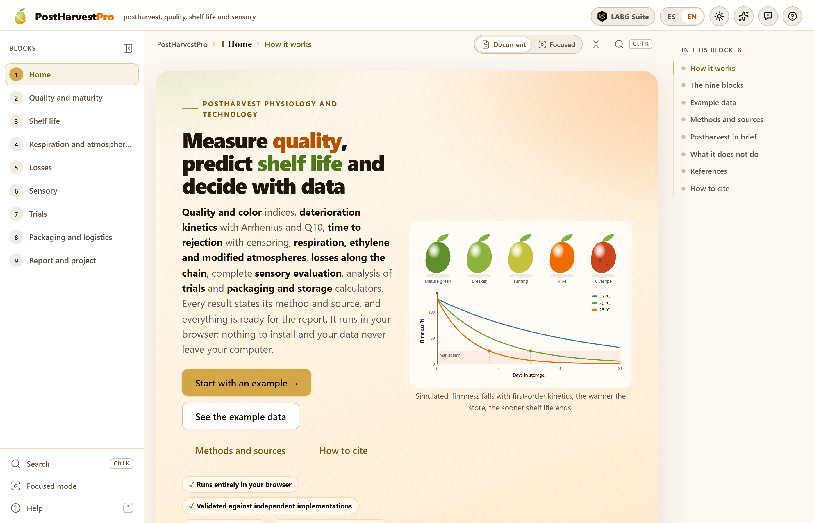
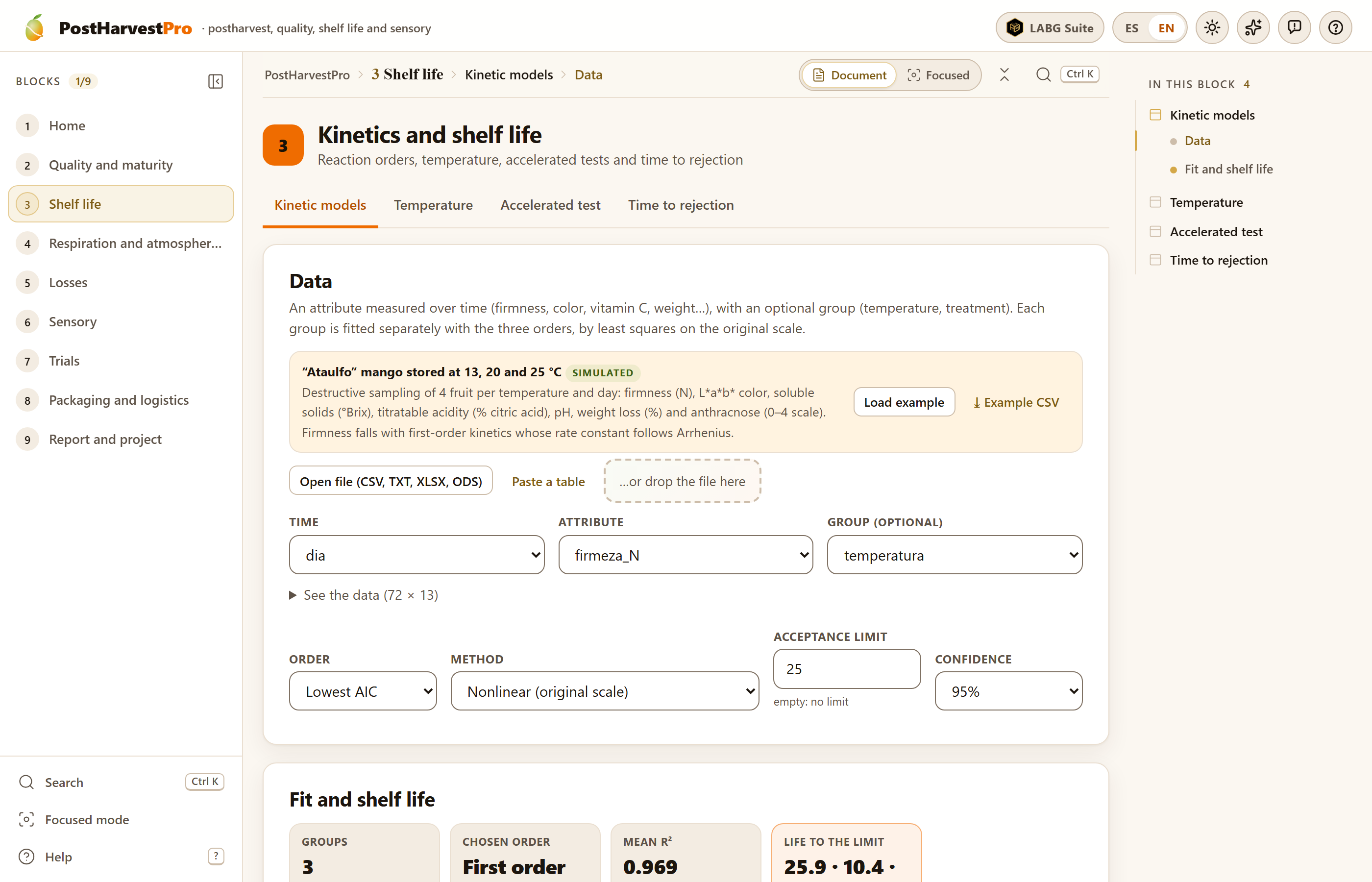 1
2
3
4
5
6
7
8
9
10
11
12